Meteorological objective analysis using multiquadric interpolation scheme over India and adjoining region

 

S. K. SINHA, M. MAHAKUR and P.N. MAHAJAN

Indian Institute of Tropical Meteorology, Dr. Homi Bhabha Road, Pune -411 008, India

 

(Manuscript received May 8, 2001; accepted in final form February 15, 2002)

 

RESUMEN

Este trabajo trata acerca del desarrollo del esquema de interpolación multicuádrica para producir campos mallados de variables meteorológicas. El resultado de la aplicación de este método con datos reales se compara con análisis del esquema de Interpolación Óptima de Gandin. Como los esquemas de interpolación óptima que usan funciones de covarianza como funciones base, el esquema multicuádrico usa funciones básicas hiperboloides radiales para acomodar datos dispersos en una malla uniforme. Este esquema produce un análisis superior comparado con el de la interpolación óptima.

 

ABSTRACT

This paper is concerned with the development of the multiquadric interpolation scheme to produce gridded fields of meteorological variables. The results of the application of this method to real data is compared with analysis from Gandhi's Optimum Interpolation scheme. Like the optimum interpolation scheme, which uses covariance functions as the basis functions, the multiquadric scheme uses hyperboloid radial basis function to fit the scattered data to a uniform grid. This scheme produces superior analysis compared to optimum interpolation analysis.

Key words: Multiquadric interpolation, optimum interpolation, hyperboloid basis function.

 

1. Introduction

The success of numerical weather prediction methods significantly depends on the production of regularly gridded data over the region concerned. A number of methods have been developed to represent scattered observation on a uniform grid. Objective analysis studies of meteorological variables started with Panofsky (1949). He attempted to produce contour lines of upper-air wind by fitting third order polynomials and employing the least square method to the observations at irregular sites. But this scheme is unstable in regions where data coverage is not uniform. Bergthorsson and Döös (1955) proposed the basis of successive correction methods. Cressman (1959) developed a number of corrected versions based on reported data within a specified distance from each grid points (R). The value of R is decreased with successive scans and the resulting field of the latest scan is taken as the new approximation. This scheme has been used for the last four decades and is empirical in nature. In recent years, this scheme has been replaced by an optimum interpolation (OI) scheme based on the ideas introduced by Eliassen (1954) and Gandin (1963). An interesting and complete summary of Gandin's work can be found in Herzfeld (1996). Here, the implied assumption is that the observations are spatially correlated. Consequently, observations that are close to each other are highly correlated. Hence, as the observations get farther apart, the regional dependence decreases. This technique employs historical data about the structure of the atmosphere to determine weights to be applied to the observations. Schlatter (1975) made multivariate objective analysis using the OI scheme, which combines mass and wind fields to produce dynamically consistent analysis, important for numerical modeling. The multiquadric interpolation (MQI) technique developed by Hardy (1971) has been widely applied in Geophysics, Geography, and Geodesy; however, its application to meteorology was very limited. Nuss and Titley (1994) applied the MQI technique to actual meteorological data and obtained a high quality of analysis. In this paper, the above technique is applied to analyse mean sea level pressure field over India and adjoining regions, and it is found that the analysis obtained using this new technique is superior to earlier analyses.

The basic mathematical theory of MQI is described in section 2. In section 3, a brief theory of optimum interpolation is presented. Data and the synoptic situation are described in section 4. Sections 5 and 6 describe the analysis experiment, and conclusions are drawn in section 7.

 

2. Methodology

Multiquadric interpolation

Hardy (1990) reviewed the basic theory of MQI. The MQI scheme using radial basis function is given by

where G(X) is the pressure field and P(X - X_i) is a radial basis function. (X - X_i) is the vector between observation point X_i and any other point in the domain. The coefficients W_i are the weighting functions. The basis function used in the OI scheme is the covariance function between the observed value and any other point in the domain of analysis. In the MQI scheme the hyperboloid function is used as a basis function, and has the form

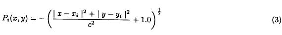
where c is a small constant and is referred to as the multiquadric parameter. This parameter (c) involved in Eqn. 2 makes the basis function infinitely differentiable by preventing the basis function to be zero at the point of observation. If X(x_i, y_i) is the position vector, then the hyperboloid function in two dimensions can be written as

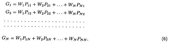
Applying the interpolation equation (Eqn. 1) to all the observation points (x_i, y_i), we get the following system of linear equations

where

Eqn. 4 holds for N observations. This results in a set of N linear equations with N weighting factors (W_i).

In matrix notation

from (7) weights W_i are obtained as follows

The inverse matrix P^-1 is solved using some standard library subroutine. It is to be noted here that the observations G(x_j, y_j) are the deviations of the observed values from some background field and after the analysis background field is added to the analysis. The interpolated values at the grid G_g, are given by

where the P_gi element of the matrix is

As stated by Franke (1982) and Kansa (1990), the MQI scheme produces most accurate results if the meteorological observations are flawless. Since meteorological observations are not error-free, errors as well as incomplete sampling of the small scale features produce unrealistic analyses. Thus, it is necessary to filter or smooth these unresolved scales from the analysis. Spatially smoothed covariance functions in the OI scheme filter out unresolved scales. In order to apply the MQI scheme to real data containing observational and other errors the Eqn. (7) has been slightly modified. The final equation in matrix form is given by

where N is the number of observations, σ² the observational error variance, θ the smoothing parameter and δ_ij is the Kronecker delta.

 

3. Optimum Interpolation Scheme

Let the scalar field f denote correlated variables such as pressure. Subscripts i and j refer to observation points and g refers to the grid point. Superscripts o and p refer to observed and background field (predicted value) respectively. N is the number of observations, denotes the value of , where the bar represents the average over number of cases. In this notation, the OI scheme is given by the following equations:

The W_j are the weights for OI corrections where the analysed values at the grid points are given by

where  represent analysed and predicted values at the grid point g. 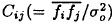is the spatial correlation coefficient, λ²(= σ²/σ₀²) is normalized observational error variance, δ_ij is Kronecker delta, σ² is observational error variance and σ₀² is back-ground error variance.

 

4. Data and synoptic situation

To examine the performance of the new scheme, mean sea level pressure on 5-8 July 1979, 00 UTC over India and adjoining regions were collected. For objective analysis using the OI scheme data on the sea level pressure gathered during the month of July for ten years (1976-1985) are used. From this data structure functions and auto-correlation functions are computed. Persistency (previous day analysis) from the Indian Meteorological Department (IMD) is used as background field. We have chosen this period because it was then that a low was formed over the head Bay of Bengal with its central region near 20°N and 90°E on 4 July 1979, and moved slowly at the beginning and intensified into a depression on 7 July, crossing the Indian coast on 8 July.

 

5. Analysis experiment

A real data experiment is carried out to judge the MQI scheme. Analyses have been performed over a region bounded by 6°N to 30°N and 60°E to 104°E with a grid resolution of 2°. In addition to the MQI, we have carried out analyses with one more interpolation scheme viz. OI scheme for comparison purpose. A nine point interpolation is applied to the background field to get the guess values at the observation locations.

Analyses and results using these two different scheme for 7 July are only presented and discussed (Figs, 1a, b). Although results for 7 July are presented, similar results are obtained for other days. The values of the multiquadric parameter (c) and smoothing parameter (θ) used are 0.001 and 0.025 respectively. For the OI analysis a Gaussian function [a. exp(-bs_ij²] is fitted to the observed correlations which are obtained on the basis of data gathered for ten years in July. The values of a and b involved in the Gaussian function are 0.793 and 0.003 respectively and s_ij is the distance between two locations. The normalized root mean square (nrms) errors between analyses (with different values of smoothing) and observations are calculated to determine the effect of smoothing and will be discussed in later section. Nrms errors are calculated in order to ensure the independence of smoothing from the type of observation. It is obtained by dividing the rms error by the variance of the pressure field. For 275 observations the variance is 6.4 hPa² about a mean of 1007 hPa. The magnitudes of nrms errors indicate how well the analysis fits the observations. The smaller the nrms error the closer is the fit of analysis to the observations. However, a closer fit to the observations need not necessarily lead to better forecast since the analysed fields have to be compatible with the dynamics as well as physical processes used in the forecast models.

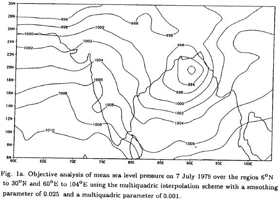
Looking at the two analyses (Figs, 1a, b) of sea level pressure using multiquadric and optimum interpolation schemes, it is observed that low pressure over north Bay of Bengal is captured well by both the schemes. The MQI produces a low pressure area with a central pressure of 993.1 hPa, while the OI produces low pressure area with a central pressure of 993.7 hPa. The IMD chart (Fig. not shown) from 7 July shows three closed isobars surrounding the centre of the depression. This is well reflected in MQI analysis carried out on 7 July, whereas in the OI scheme only two closed isobars are seen. The nrms difference of MQI and observations on 7 July is 0.074 hPa^-1, whereas in the case of OI scheme the error is 0.137 hPa^-1.

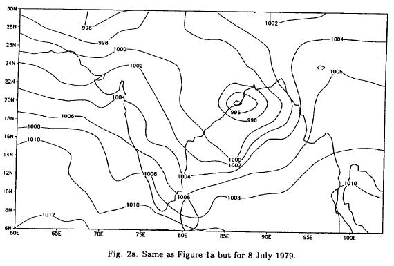
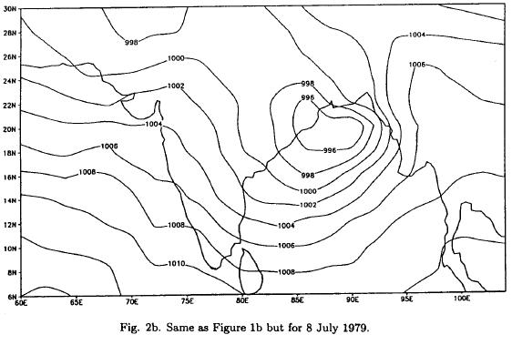
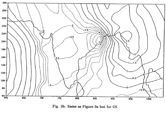
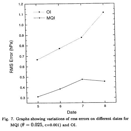
Table 1 shows the rms and nrms differences on all days. It is found that errors in the MQI scheme are considerably less when compared to the OI scheme. On an average, there is a reduction in error by about 52%. This difference is large on 8 July (about 59%). It is interesting to note that on 8 July the centre of the depression was located at 20°N, 86.5°E (IMD chart, Fig. not shown) whereas in the MQI and the OI schemes the locations of the centre of the depression were at 20°N, 86°E and 20°N, 90°E respectively (Figs. 2a, b). Thus, we find that the MQI analysis is closer to the IMD analysis. Figures 3(a, b) show the analysis of the total corrections at individual grid points for MQI and OI for 8 July 1979. It is observed that at grid point 20°N, 86°E the total corrections to the initial field in the analysis of MQI is -5.8 hPa, whereas in the analysis by OI it is -4.6 hPa. Thereby, the central pressure for MQI is reduced to 993.4 hPa, whereas in the case of OI it becomes 994.6 hPa. Again, it is observed that total corrections at grid point 20°N, 90°E is 5.3 hPa and 0.9 hPa in the case of MQI and OI respectively. The initial guess field for 8 July at grid point 20°N, 90°E, which is 993.0 hPa, is substantially modified, whereas the modification in the initial field for OI scheme is much lower. Hence the depression located at 20°N, 90°E remains stationary in OI analysis, whereas for MQI it is shifted to 20°N, 86°E, which resembles that obtained during the IMD analysis.

With θ = 0.0 (unsmoothed) the MQI scheme produces low pressure area with a central pressure of 993 hPa (Fig. 4) with nrms difference 0.073 hPa^-1. These differences between the analyses indicate the characteristics of the MQI scheme. In fact MQI scheme with θ = 0.0 (unsmooth) should exactly fit the observations (nrms=0). But this is not so because errors occur during the back interpolation from the analysis to the observation locations.

 

6. Effect of different parameters

Smoothing parameter

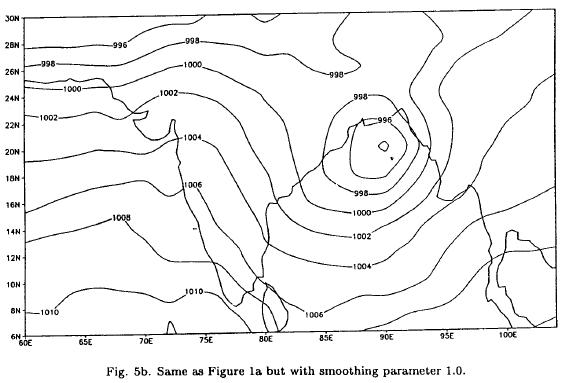
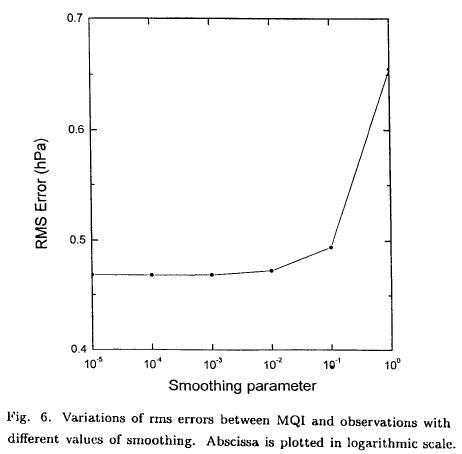
As stated by Nuss and Titley (1994), the smoothing parameter (θ) in the MQI scheme (Eqn. 11) is a measure of the least square fit. To show the effect of the smoothing parameter (θ) on the analysis, experiments have been carried out with different values of θ, ranging from 10^-5 to 1.0. Analyses with θ = 0.1 and 1.0 are shown in figures 5(a, b). It is observed that a low pressure centre with a pressure of 993 hPa (θ = 0.0) reaches 993.2 hPa for θ = 0.1 and 993.6 hPa for θ = 1.0. Rms errors are computed for determining the quantitative effect of smoothing parameter. Figure 6 shows the variation of rms differences with smoothing parameters over a range of 10^-5 to 1.0. It is observed that up to θ = 10^-3 there is no change in the rms error, but after θ = 10^-3 errors increase with increasing values of smoothing parameter and reach up to 0.66 hPa for θ = 1.0. Figure 7 shows the variations of rms errors on different days for the MQI and the OI schemes.

Multiquadric parameter

The multiquadric parameter (c) in Eqn. (2) determines the curvature of the basis function, i.e., the hyperboloid. A large value of c corresponds to a small curvature (flat hyperboloid), whereas a small value of c corresponds to large curvature. For the basis function to have a continuous derivative, c should be non-zero. Although the value of multiquadric parameter c influences the analysis, but the interpolation is not too sensitive to the exact value of c. Hardy (1990) tested the sensitivity of the multiquadric scheme by varying the value of c from 0.000005 to 0.5. He found that the coefficient matrix remained well conditioned for c = 0.5, which is the upper limit of c for the set of observations which he has used. For the present set of observations which are used in this analysis, we typically used c = 0.001. Computational stability when solving Eqn. (11) for weighting functions depends on the multiquadric parameter (c). If c² is large and the argument in the radial basis function (Eqn. 1) (X - X_i)² is small, then the matrix in Eqn. (11) has equal diagonal and off diagonal elements which yield an ill conditioned matrix. Thus, the multiquadric parameter has great influence on the analysis. Figure 8 shows the variation of rms errors with different values of c. The analysis is done on a unit domain with c = 0.001. Analyses are transformed to a unit domain where x and y vary from 0.0 to 1.0 for practical purposes.

 

7. Conclusions

The multiquadric interpolation scheme is simple and can produce analysis with minimum smoothing, and it is more accurate than the Gandin (1963) OI scheme. It is a 2-dimensional univariate analysis scheme and can be easily extended to a 3-dimensional analysis by simply adding another term (z - z_i)² in Eqn. 3. IMD analyses of 4 to 7 July 1979, 00 UTC have been used as background field. A non-zero value of c is essential to ensure the continuous derivative of the basis function. Since the basis function is continuously differentiable, a dynamic relationship can be applied to this scheme to simultaneously analyse mass and wind fields.

 

Acknowledgements

The authors would like to thank Dr. G. B. Pant, Director, Indian Institute of Tropical Meteorology, Pune for his interest and providing the necessary facilities to carry out this study, and Dr. S. S. Singh, Head, FRD for his encouragement. The authors are most thankful to the anonymous reviewers for their valuable comments and suggestions. Thanks are also due to the Indian Meteorological Department for providing the necessary data.

 

REFERENCES

Bergthorsson, P. and B. R. Döös, 1955. Numerical weather map analysis. Tellus, 7, 329-340.         [ Links ]

Cressman, G. P., 1959. An operational objective analysis system. Mon. Wea. Rev., 87, 367-374.         [ Links ]

Eliassen, A., 1954. Provisional report on calculation of spatial covariance and autocorrelation of the pressure field. Inst. Weath. and Climate Res. Acad. Sci. Oslo, Report No.5, 1-11.         [ Links ]

Franke, R., 1982. Scattered data interpolation: Tests of some methods. Math. Cornput., 38, 181-200.         [ Links ]

Gandin, L. S., 1963. Objective analysis of meteorological fields. Translated (1965) from Russian by Israel Programme for Scientific Translation, Jerusalem, 242 pp.         [ Links ]

Hardy, R. L., 1971. Multiquadric equations of topography and other irregular surfaces. J. Geophys. Res., 76, 1905-1915.         [ Links ]

Hardy, R. L., 1990. Theory and applications of the multiquadric - biharmonic method. Comput. Math. Appl., 19, 163-208.         [ Links ]

Herzfeld, U. C, 1996. Inverse theory in Earth science - an introductory overview with emphasis on Gandin's method of optimum interpolation. Math. Geol., 28, 137-160.         [ Links ]

Kansa, E., 1990. Multiquadrics - A scattered data approximation scheme with application to computational fluid dynamics. I: Surface approximations and partial derivative estimates. Comput. Math. Appl., 19, 127-145.         [ Links ]

Nuss, W. A. and D. W. Titley, 1994. Use of multiquadric interpolation for meteorological objective analysis. Mon. Wea. Rev., 122, 1611-1631.         [ Links ]

Panofsky, H. A., 1949. Objective weather map analysis. J. Meteor., 6, 386-392.         [ Links ]

Schlatter, T., 1975. Some experiments with a multivariate statistical objective analysis scheme. Mon. Wea. Rev., 103, 246-257.         [ Links ]