On atmospheric energy cascades

 

A. WIIN-NIELSEN

The Collstrop Foundation, H.C. Andersens Blvd. 37 DK 1553 Copenhagen V, Denmark

 

(Manuscript received February 8, 2001; accepted in final form June 1, 2001)

 

RESUMEN

Los términos de advección en las ecuaciones atmosféricas de movimiento resultan, en el dominio espectral, en un intercambio entre los varios números de onda de energías potencial y cinética que están disponibles. Estudios observacionales han demostrado que mientras la energía potencial disponible es llevada en cascada de números de onda menores a mayores, la energía cinética es también llevada en cascada de los números de onda intermedios hacia, tanto los números de onda altos, como los bajos debido supuestamente al hecho de que la conversión de energía disponible a energía cinética es grande en un intervalo de la escala del número de onda.

El propósito de este artículo es reproducir algunos aspectos mayores de estos procesos de transporte de energía en cascada, usando primero un modelo extremadamente simple basado en un fluido homogéneo con una superficie libre. El factor conductor en el modelo es agregar y sustraer fluido de tal modo que la adición neta se anule. El modelo estará además restringido a una dimensión espacial en la dirección oeste-este, reteniendo las no linearidades en los términos de advección.

Las ecuaciones del modelo que contienen forzamiento y disipación son integradas numéricamente hasta el estado estacionario. Evaluaciones de la generación de energía, convecciones y disipaciones, demuestran que el modelo de procesos en cascada se comporta correctamente con respecto a la dirección y magnitud comparado con otras conversiones de energía en el modelo, y es cualitativamente correcto comparado con estudios observacionales.

El segundo modelo se basa en las ecuaciones primitivas para los dos componentes horizontales del viento y en la ecuación termodinámica que incluye un calentamiento específico que es independiente del tiempo. Este modelo es también tratado en la dirección zonal, únicamente y en el espacio del número de onda. El modelo da buenas simulaciones de la transferencia, tanto de la energía potencial y la energía cinética disponibles, como funciones del número de onda.

 

ABSTRACT

The advection terms in the atmospheric equations of motion will in the spectral domain result in an exchange of available potential and kinetic energies between the various wave numbers. Observational studies have demonstrated that while the available potential energy cascades from lower to higher wave numbers, the kinetic energy is cascaded from the middle wave numbers to both the high and the low wave numbers supposedly due to the fact that the energy conversion from available potential energy to kinetic energy is large in an interval of the wave number scale.

The purpose of the present paper is to reproduce some major aspects of these energy cascade processes using first an extremely simple model based on a homogeneous fluid with a free surface. The driving factor in the model is the use of adding and subtracting fluid in such a way that the net addition vanishes. The model will furthermore be restricted to one space dimension in the west-east direction retaining the nonlinearities in the advection terms.

The model equations, containing forcing and dissipation, are integrated numerically to a steady state. Evaluations of the energy generation, conversions and dissipations show that the model cascade processes behave correctly with respect to direction and magnitude as compared to the other energy conversions in the model and qualitatively correct compared to observational studies.

The second model is based on the primitive equations for the two horizontal wind components and the thermodynamic equation including a specified heating which is independent of time. This model is also treated in the zonal direction only and in wave number space. The model gives good simulations of the transfer of both available potential and kinetic energy as functions of the wave number.

Key words: energy cascades, nonlinear exchanges.

 

1. Introduction

The nonlinear cascade processes were evaluated by Saltzman and Teweles (1964) and by Yang (1967) from atmospheric data, where the first authors used a data set covering nine years with a low vertical resolution, while Yang used data for one year only with many levels in the vertical direction. The observational studies were described by Steinberg et al. (1971). The formulation of these energy conversion integrals was done in detail for the spherical case by Wiin-Nielsen and Chen (1993, see chapter 10) containing also the main results of the observational studies dividing the waves in three groups: the long waves (wave numbers 1-5), the middle waves (6-10) and the short waves (11-15). For the eddy available potential energy it was found that the cascade goes from the very long waves to the middle long and the short waves, while the cascade of the kinetic energy goes from the middle long waves to both the long and the short waves. The exchange of the energies among the three groups are small compared to the total eddy conversion from the available potential to the kinetic energy.

To simulate these processes we shall first use a model of a homogeneous fluid with a free surface. Simulating the heating of the atmosphere we shall imagine a process whereby fluid is added and subtracted in various regions with the net-addition being zero. Such a process will generate available potential energy, which may be converted to kinetic energy on the various wave numbers. We shall then investigate the cascade processes of the kinetic energy and compare it with the observational studies.

In the atmosphere we have a maximum growth of the kinetic energy in the middle wave numbers due to the barotropic and baroclinic instabilities on these scales. Such processes may (in the simple model employed here) be simulated by a large addition of fluid in these middle scales. The cascade processes in the model will distribute the added energy to the other scales.

Since the cascade processes originate from the advection processes, and since these processes consist of a multitude of interactions, each involving three wave numbers, we cannot linearize the model. Consequently, it is necessary to employ numerical integrations which may approach a steady state after a sufficiently long integration. To keep the model as simple as possible, we shall consider changes in the west-east direction only. The basic equations are thus the continuity equation containing the forcing and the two equations of motion for the horizontal wind components.

The second model is based on the two primitive equations for the horizontal wind components and on the thermodynamic equation containing the heating in the model.

 

2. The model equations for the first model

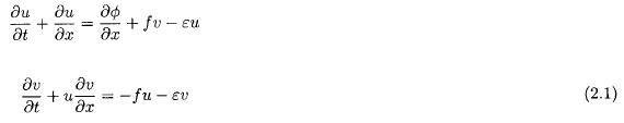
Based on the formulation of the model as described in the introduction we shall use the two equations of motion in the form displayed in (2.1).

In (2.1) we have used a simple form of the frictionál term. Another choice would have been to use a diffusion term proportional to the second derivative of the wind component. A number of integrations using such a term were carried out. It appears that while the time integrations can be carried out the strong dependence on the wave number in the dissipation term gives a too large dissipation for large values of the wave number.

To keep the model as simple as possible, we shall employ the continuity equation in the form given in (2.2).

It was decided to disregard the advection term on the left hand side of (2.2) since its contribution is small due to the small u-values in the results.

In case we had included this advection term, it would have been necessary for consistency to include an additional term in the expression for the divergence. The forcing S(x) has the dimension of m per s, and we may visualize S(x) as representing the addition and subtraction of fluid.

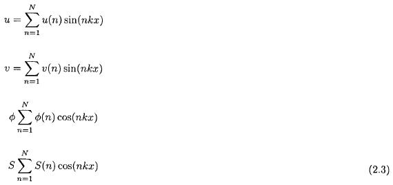
In order to integrate these equations numerically, it is an advantage to formulate the equations in the spectral domain. One could include both sine and cosine terms in the series for the dependent variables, but the equations are easier to handle if we introduce just one trigonometric function in each of the variables. Let us therefore suppose that we apply the equations at a given latitude (say 45 degrees north). We may then write u and v as a sum of sine functions, while the geopotential and the forcing will be written as series of cosine functions as shown in (2.3), in which k = 2π/L where L = 28000 km is the approximate length of the latitude circle at 45 degrees North.

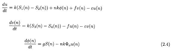
The three spectral equations may then be written as given in (2.4).

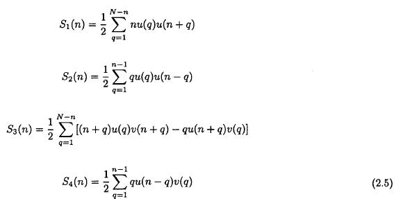
The four sums appearing in (2.4) are defined in (2.5) as derived by Wiin-Nielsen (1998).

The forcing applied in this simple model should simulate the conversion of available potential to kinetic energy. We know that the largest part of this energy conversion takes place at the middle wave numbers due to barotropic and baroclinic instability. It is this process that we try to simulate rather than the heating in the atmosphere. To simulate the heating itself we need to use a baroclinic model with at least two levels as done later in this paper.

 

3. Numerical integrations of the equations of the first model

The numerical integrations are carried out using the Runge-Kutta procedure, and they are continued to a time, where a steady state has been reached. The initial state could have been a state of rest with vanishing geopotential, but if this is done, it would require a very long integration to reach a steady state. The initial state is defined using the three model equations in (2.4). The zonal wind is determined from the third model equation as given in (3.1).

The meridional component is determined from the second equation, in (2.4) by disregarding the contribution from the two nonlinear sums. We obtain then the formula shown in (3.2).

The initial value of the geopotential is finally determined from the first equation in (2.4) as shown in (3.3).

From the initial state defined above, the equations are integrated to a steady state. It is normally reached after an integration of about 50 days.

Figure 1 shows the forcing applied in the first integration. It is seen that the forcing is defined with a maximum at wave number 7 and with decreasing values for both smaller and larger wave numbers. The particular specification is shown in (3.4).

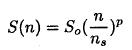
where the top formula is valid for n < n_s and the bottom formula for n > n_s

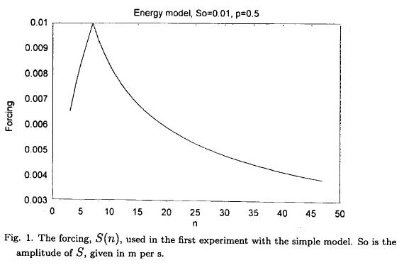
Figure 2 shows a part of the energetics for the steady state after an integration with p = 1/2. The solid curve is the generation of available potential energy. The marks on this curve indicate the energy conversion from available potential to kinetic energy. The two quantities are the same because of the steady state balance in the third equation of motion. The dotted curve is the dissipation of the kinetic energy. This curve is different from the other two because the two equations of motion also contain the cascade processes depending on the four sums in these equations i.e. the nonlinear energy transfer in the spectrum.

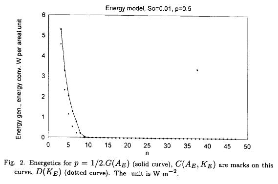
The difference between the two curves is then a measure of the interaction among the wave components. The same result can be illustrated in a better way by calculating a flux-function defined as shown in (3.5).

where the right hand side is the energy conversion to a given wave number from all the nonlinear interactions affecting wave number n. The integration of (3.5) contains a constant which may be calculated by noting that the mean value of the flux-function over all wave numbers is zero. Figure 3 shows the result which indicates that the flux of kinetic energy in the spectrum is toward the longer waves for small values of n, while the flux for the larger values of n is toward the larger wave numbers. This result is in agreement with the main result obtained from observational studies.

A second example follows. The forcing is in this case defined as shown in (3.6).

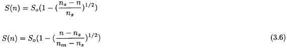
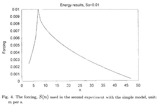
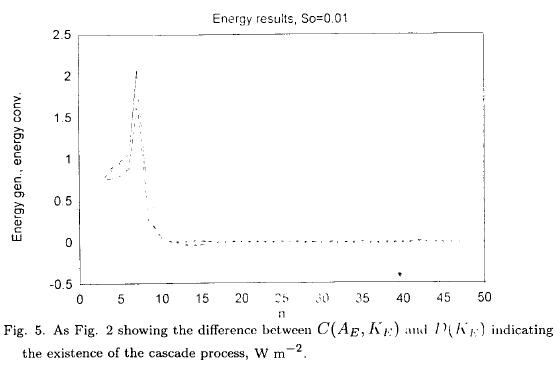
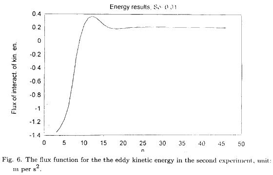
Figure 4 shows the forcing which, as before, has a maximum for n = ns = 7. Figure 5, corresponding to Figure 2, shows as in the first case, a difference due to the cascade processes. Figure 6 contains the flux-function. While different from the fluxfunction given in Figure 3, it still shows negative values for the small values of the wave number and positive values for the larger wave numbers. The flux is thus in qualitative agreement with the observational studies.

 

4. The second model

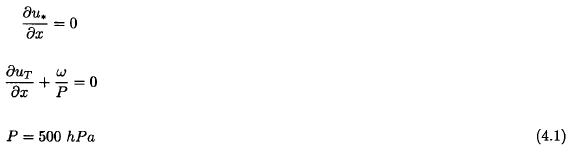
The model is based on the general two-level model, but it is here reduced to equations valid for the x-direction only. We may start by considering the continuity equation with the boundary conditions: the vertical p-velocity, ω vanishes at the top of the atmosphere and at the isobaric surface close to the ground, i.e. at 1000 hPa. Using the subscripts 1 and 3 for the isobaric surfaces with pressures 250 and 750 hPa and the subscripts * and T for half the sums and half the differences between variables at these surfaces, we obtain from the continuity equation the expressions given in (4.1). The interpretation of the first of these equations is that the zonal velocity at the level * is constant. We may set this constant to any value, and we prefer to set it equal to zero.

The four equations of the model may then be written as expressed in (4.2).

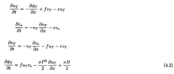
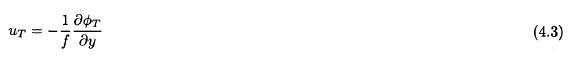
In these equations we have used the continuity equation to eliminate the vertical p-velocity from the thermodynamic equation. We have furthermore eliminated the south-north derivative of the geopotential by using the geostrophic relation given in (4.3).

This relation is difficult to justify in advance, but as it turns out after the integrations with respect to time, the state of the model is quasi-geostrophic.

As in the simple model, we shall replace the four equations given in (4.3) by the corresponding spectral equations using again sine functions for the velocity components and cosine functions for the geopotential and the heating appearing in the last of the four equations. The nonlinear terms appearing in the last three equations will, as in the previous case, lead to sums which have to be calculated in each timestep.

The spectral equations may be written in the form shown in (4.4) in which we have introduced the constants: st = σP²/2 and k = R/c_p.

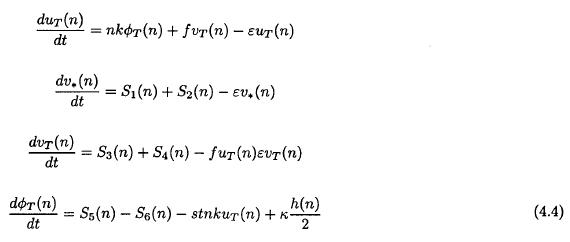
The last three equations contain each two nonlinear sums. They have been determined, as in the other cases, by calculating the integrals of the triple product of the trigonometric functions. The sums are listed in (4.5).

As in the simpler model treated above, it will also in this case be necessary to define a reasonable initial state. This process starts by disregarding the nonlinear sums in the thermodynamic equation. We may then obtain the determination shown in (4.6).

Neglecting again the nonlinear sums the third equation in the system leads to (4.7).

The second equation provides v_*(n) = 0. From the first equation we may then obtain an expression for the thermal geopotential as shown in (4.8).

The selected initial state, given in (4.6), (4.7) and (4.8), is far from the steady state solution of the four nonlinear equations, but it is better than starting from an initial state of rest with no gradient in the geopotential field.

 

5. Numerical integrations of the model equations for the second model

The numerical integrations are carried out using the same numerical scheme as in the first model. A time step of 5 minutes was selected, because larger values resulted in numerical instabilities. It turns out that the integrations approach the desired steady state in a very slow manner. To obtain an accurate determination of the steady state, it is necessary with the selected initial state to continue the numerical integrations for 300 days although integrations covering 200 days give reasonable approximations. In addition, the cascade processes which are the major processes treated in this paper, appear before the steady state is reached. The flux functions for the two kinds of energy will therefore be shown for some states during the integrations,

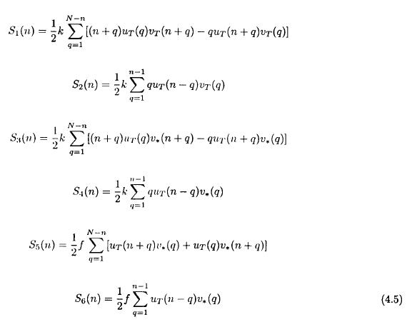
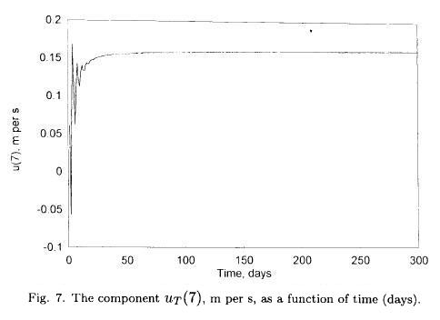
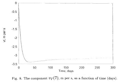
Figure 7 shows that the component u_T(7) reaches the equilibrium value after only 50 days. On the other hand, Figures 8 and 9, showing the time variations of the seventh component of v_T and Φ_T illustrate a very slow approach to the steady state.

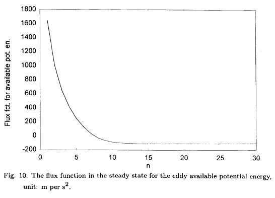
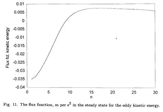
The main results obtained with the second model are presented in Figures 10 and 11. The first of these two figures, giving the flux function for the available potential energy as a function of the wave number, confirms the studies of the first model indicating that the eddy available potential energy is cascading from the very long waves to the shortest waves in the model. The second of these two figures, giving the flux of eddy kinetic energy as a function of wave number, indicates a flux from middle long waves to the very long waves, while the decreasing part of the curve shows an energy flux toward the shortest waves in the model.

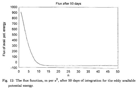
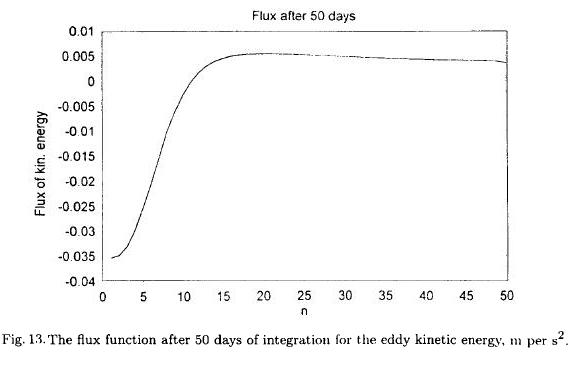
Figures 12 and 13 contain the same information as Figures 10 and 11, but after only 50 days of integration. It is seen that these flux functions are of the same nature as those obtained from the steady state.

It should also be mentioned that due to the assumption of permitting only variations in the zonal directions we have assumed that the zonal wind component at the middle level (500 hPa) is equal to zero. It follows from this assumption that the equation for this zonal component reduces to a diagnostic equation as given in (5.1).

This equation permits the determination of the geopotential at 500 hPa because the thermal u-component and the v-component at 500 hPa are known from the time-integration of the four prognostic equations given in Section 4.

The equation (5.1) was formulated in the spectral domain with the results given in (5.2).

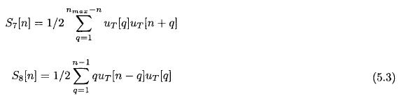
The two sums appearing in (5.2) are shown in (5.3).

The geopotential at the middle level was calculated in wave number space using (5.2) and (5.3) at the end of a time integration. It is seen from (5.2) that an approximate geostrophic adjustment will exist at the middle level if the two sums are small compared with the remaining two terms. The geostrophic component was therefore computed from the knowledge of the geopotential at the middle level and compared with the same component in the model integration. It turns out that the geostrophic adjustment is almost perfect.

 

7. Conclusions

The main result of the investigations of cascade processes using simple barotropic and baroclinic models with forcing and dissipation and restricted to the west-east direction is that the models, after integration with respect to time, produce cascade processes which are in good agreement with the calculation of the same processes from observed data. The calculated nonlinear interactions also agree with observational studies in the sense that the energy conversions due to the cascade processes are numerically small compared to the the total generation of available potential energy created by the heating incorporated in the model.

 

REFERENCES

Saltzman, B. and S. Teweles, 1964. Further statistics on the exchange of kinetic energy between harmonic components of the atmospheric flow, Tellus, 16, 432-435.         [ Links ]

Steinberg, H. L., A. Wiin-Nielsen, C.-H. Yang, 1971. On nonlinear cascades in large-scale atmospheric flow, Jour. of Geophys. Res., 76, 8629-8640.         [ Links ]

Wiin-Nielsen, A. and T.-C. Chen, 1993. Fundamentals of atmospheric energetics, Oxford Univ. Press, 376 pp.         [ Links ]

Wiin-Nielsen, A., 1998. On the spectral distribution of kinetic energy in large-scale atmospheric flow, Nonlinear Processes in Geophysics, 5, 187-192.         [ Links ]

Yang, C.-H., 1967. Nonlinear aspects of the large-scale motion of the atmosphere, Ph. D. diss., Univ. of Michigan, 173 pp.         [ Links ]