Linear and regressive stochastic models for prediction of daily maximum ozone values at Mexico City atmosphere

 

J. L. Bravo

Instituto de Geofísica, UNAM, Circuito Exterior, CU, 04510, México, D. F., México

 

M. M. Nava

Instituto Mexicano del Petróleo, Gerencia de Ciencias del Ambiente, Eje Central Lázaro Cárdenas No. 152, Apartado postal 14-805, 07730, México, D. F. México

 

C. Gay

Centro de Ciencias de la Atmósfera, UNAM, Circuito exterior, CU, 04510, México, D. F., México

 

(Manuscript received Feb. 21, 2000; accepted in final form Oct. 16, 2000)

 

RESUMEN

Se aplica un procedimiento basado en la metodología conocida como ARIMA, para predecir, con 2 ó 3 horas de anticipación, el valor máximo de la concentración diaria de ozono. Está basado en el cálculo de autorregresiones y promedios móviles aplicados a los valores máximos de ozono superficial provenientes de 10 estaciones de monitoreo atmosférico en la Ciudad de México y obtenidos durante un año de muestreo. El pronóstico para un día se ajusta con la información meteorológica y de radiación solar correspondiente a un periodo que antecede con al menos, tres horas la ocurrencia esperada del valor máximo. Se compara la importancia relativa de la historia del proceso y de las condiciones meteorológicas previas para el pronóstico. Finalmente se estima la probabilidad diaria de que un nivel normativo o preestablecido para contingencias de ozono sea rebasado.

 

ABSTRACT

We developed a procedure to forecast, with 2 or 3 hours, the daily maximum of surface ozone concentrations. It involves the adjustment of Autoregressive Integrated and Moving Average (ARIMA) models to daily ozone maximum concentrations at 10 monitoring atmospheric stations in Mexico City during one-year period. A one-day forecast is made and it is adjusted with the meteorological and solar radiation information acquired during the first 3 hours before the occurrence of the maximum value. The relative importance for forecasting of the history of the process and of the meteorological conditions is evaluated. Finally an estimate of the daily probability of exceeding a given ozone level is made.

 

1. Introduction

In this work we aim at establishing a procedure to forecast, with a lead time of 2 to 3 hours, maximum daily surface ozone concentrations in the Mexico City Metropolitan Area (MCMA), using linear stochastic and multiple regression models. The risk of exceeding limits, like those established by environmental authorities is evaluated in order to take opportune warnings and actions to restrict the emissions of ozone precursors to the atmosphere.

High tropospheric ozone concentrations are a man-made phenomenon. Ozone is a secondary pollutant formed in urban areas and its vicinities as a result of the photolisis of nitrogen oxides (NOx) in presence of non methane hydrocarbons (NMHC) and other organic compounds (Finlayson-Pitts and Pitts, 1986, Böhm et al., 1991).

Ozone, at concentrations frequently observed during pollution episodes in urban areas, is harmful for humans, animals and plants (Campos et al., 1992; Quadri and Sánchez, 1992; NRC, 1991). Inside big cities the period of exposure to high concentrations is long and poses some risk for people with heart and respiratory problems. Healthy individuals can exhibit respiratory discomfort as well as irritation of the eyes (McColister and Wilson, 1975).

In Mexico City a program for decreasing the vehicular and industrial emissions during environmental contingencies was set up since November 1989. The regulations include the so-called one day without a vehicle and two days without a vehicle for cars and other vehicles. The circulation of vehicles is restricted according to registration plate ending numbers depending on the observed ozone maximum values. Other regulations limit industrial and governmental activities during high pollution episodes. On these occasions even the activities of school children are restricted to indoors, to protect them against the effects of ozone by reducing their exposure to the gas. The implementation of a program to reduce the number of these extreme events, at the end becomes a burden for the citizens. Hence predicting maximum values can contribute to planning and better relations between authorities and the public.

Two approaches have been used to predict air quality conditions. Both require information about the concentrations of primary pollutants and meteorological data. The first one relies on modeling the chemistry of the atmosphere using information obtained from controlled experiments carried out in smog chambers adjusted to atmospheric conditions and using dynamical models to obtain the future behavior of the atmosphere. Although this is a logic approach, there are difficulties in handling or getting the necessary large amounts of emission data and also in the consideration of all theoretical aspects, many of them oversimplified and far from the real conditions. When these problems persist the precision and reliability of the forecast is reduced (Chock et al., 1975).

The second approach consists in modeling ozone concentrations by means of the statistical analysis of existing data, complemented by knowledge of the basic physical and chemical processes occurring in the atmosphere. This approach is the basis of this work. Statistical models can give reliable results, when they are built with good continuous sets of data. The reliability of the results is not guaranteed when the data are extrapolated out of the range of values used in the adjustment of the model (Chock et al., 1975). Only a few works have been published with this semi-empirical approach of forecasting for the MCMA (Bravo et al., 1996; Castañeda, 1997; Cuevas, 1997).

The use of statistical methods sometimes needs conditions that in occasions are difficult to fulfill (for example normality and independence of the input data), especially in the cases when the data have strong autocorrelation. The existence of strong autocorrelations in climatic and air quality data is well known. Then it is necessary to consider atmospheric processes as stochastic. Several authors (Castañeda, 1997; Cuevas, 1997; Milions and Davies, 1994a, 1994b) have used the Box and Jenkins (1976), technique to carry out univariate and intervention analysis to forecast and evaluate the pollutant time series structural changes, due to the effects of external events like several actions taken by the Mexican petroleum industry and environmental authorities in the fuels changes and reformulation.

In the present study the methods proposed by Box and Jenkins (1976); Box and Tiao (1975) and González (1990) known as autoregressive integrated and moving average (ARIMA), or linear stochastic models, were adjusted to daily maximum of hourly tropospheric ozone concentrations obtained at 10 monitoring sites.

ARIMA models use past values of a time series and past random errors to predict future values. After the identification and fitting of an ARIMA model, we assumed that all the historic useful information of the process was taken into account, then the residuals of the model (errors) could be explained by the meteorological information corresponding to the moment of the observation. The residuals of the ARIMA model are adjusted to a multivariate regressive model (Draper and Smith, 1981) because they are samples of an independent random variable. The independent variables are meteorological parameters measured at one station, such as total solar radiation, or mean wind speed or nitrogen oxides concentrations measured at each monitoring site. To test the skill of the forecasting method after fitting the models, we produced a daily prediction for a month and the forecasted values were compared with the observations at the monitoring sites. The probability of exceeding certain limit values, for instance, those established by the environmental authorities, was also calculated.

 

2. Area of study

Mexico City is located in a valley surrounded by mountains that restrict free wind circulation. This facilitates the accumulation of vehicular and industrial emissions. The Valley of Mexico is located at 2268 masl in a tropical zone, subjected to high solar radiation that promotes the formation of photochemical pollutants, among which ozone is the most abundant.

The ozone concentration at the MCMA shows daily variation patterns that are typical of big cities, they are bell shaped with minimum values at night, increasing after sunrise and reaching a maximum during the afternoon hours (Böhm, 1991; NRC, 1991). Downwind from urban centers, the ozone pattern reaches its maximum later in the afternoon. On the other hand, the maximum of the ozone precursors, nitrogen oxides and hydrocarbons, occur in the first hours of the morning, coinciding with the emissions of the vehicular traffic due to people being transported to their jobs.

 

3. Data and forecasting procedure

The data were obtained from 10 sampling stations selected from the Red Automática de Monitoreo Atmosférico (RAMA) (Atmospheric Monitoring Automatic Network), of the Gobierno del Distrito Federal (GDF). The stations were chosen in such a way that two of them were located in each of the five areas in which the MCMA is divided for the purpose of reporting air quality (NE, SE, SW, NW and CEnter or Downtown). The location of stations is shown in Figure 1. The examined period was the year of 1996.

The ozone data base manager employed was SOMOD (IMP, 1992) and the computational system was SIMEDA (IMP, 1995) available at the Instituto Mexicano del Petróleo (IMP). To construct the time series the hourly averages were calculated for each station during the diurnal period, and then, daily maximum values were selected. The adjustment of the ARIMA and the multiple regression models were carried out with STATISTICA (Statsoft, 1994).

The data for NO₂ and the mean magnitude of wind speed for the period 0 to 13 hours for each site were also obtained. Total solar radiation, integrated from 6:00 to 13:00 hours, measured in the Solar Radiation Observatory of the Institute of Geophysics was used. This observatory is located to the Southwest of Mexico Valley near to the Pedregal station, inside the National University Campus (UNAM). The instrument used was a Kipp & Sonen piranometer calibrated against international standards. For this work 13:00 hours was the upper limit in the selection of the meteorological information since ozone has maximum values 2 to 3 hours later as stated by Bravo et al. (2000).

The forecast was accomplished using two types of models, the first is the adjustment of ARIMA models to data series and the second was the adjustment of a multivariate linear model to the residuals of the previous model. Using these two steps procedure it is possible to evaluate separately the effect of the history of the series and the effect of the meteorological conditions the day of the observation.

A natural logarithm transformation was applied to ozone series to obtain not skewed normal distributed residuals and to fix greater than zero forecasting values and their confidence intervals. The analysis of the autocorrelation and partial autocorrelation functions of the transformed series shows high values corresponding to small lags, these values decrease smoothly with increasing lags which means that the series have a trend. The graphs of the series suggest a seasonal variation with low values during the rainy season, therefore, to eliminate the effect of trend and season, the transformed series were differentiated using the formula

where B is the backward shift operator (B(𝓍_t) = 𝓍_t—1), and 𝓍_t—1 are the natural logarithm of the ozone concentrations at day t and t — 1 expressed in parts per million. After applying these transformations the new series y_t was considered, their autocorrelation and partial autocorrelation functions look like functions from a stationary series, then an ARMA (1,1) model was identified and adjusted to all stations. The following expression defines the model

where (1 — 𝜙B) and (1 — 𝜃B) are the autoregressive and moving average polynomials respectively, ε_t is the random noise series that represents the random part of the process and μ is the mean of the y series. The coefficient Φ represents the linear influence of the one-day backward value of the series and θ represents the influence of the one-day backward of the random error of forecast into the forecast of the series. The model could be expressed as

and transformed to

which is an infinite expansion where the coefficients represent the influence of the past into the present. The objective of expressing the model in forms (2) and (3) is to obtain recurrence finite formulas that allow prediction like equation (2) instead of an infinite expansion like equation 4.

From equation (2), substituting y_t from (1), it is possible to obtain

where 𝓍_t and are the predicted and observed natural logarithms of the ozone maximum values expressed in parts per million at day t, ε_t is the forecasting error at day t, and c, 𝜙 and θ are the parameters already mentioned, determined by the adjustment of the model.

Table 1 shows the values of the parameters obtained after the adjustment and the number of data used. The correlograms of the residuals did not show significance, i. e., the correlation was not higher than that shown by white noise. Thus the residuals were treated as random independent variables.

Since the historical information about the processes is considered after fitting the ARIMA model, the residuals should not contain information that could be predicted by means of the history of the processes. Therefore, will be assumed that errors are due to the variations of all meteorological variables that affect the ozone concentrations at the time of observation. Then the residuals, after fitting the model, should be a function of the variables that modify the maximum ozone concentrations the day of the observation.

It is well known that many factors can affect the ozone concentration in a specific place and day, among them the topography, which does not vary with the time but retains the pollutant dispersion and determines part of the differences in concentrations among stations. Another factor that remains more or less constant is the type of emissions since the rural, urban or industrial areas will stay the same for some time.

The factors, that could modify the results and change everyday, are those related to meteorological conditions and weekly city's activities, for instance the weekend break. During these days pollutant emissions to the atmosphere could decrease as suggested by Bravo et al. (1996). However, in this study, the autocorrelation and partial autocorrelation functions do not support this hypothesis. Probably the amplitude of the weekly city activities effect decreased and the meteorological variations masked its presence. This could also be due to the permanent program "one day without a vehicle in the MCMA, since it allows the circulation of all vehicles on Saturday and Sunday, increasing vehicle circulation during the weekend, this implies more traffic than in Bravo et al. (1996) study. Therefore meteorological variables should explain most of the daily ozone variability.

The variables that affect the ozone concentrations are those related with the formation and dispersion or accumulation, such as the solar radiation, precursor gases and meteorological conditions. We propose the maximum hourly averages concentration of NO₂ occurring between 0:00 and 13:00 hours as an indicative variable of precursor gases, while we consider wind speed as a surrogate variable for atmospheric stability. In other words, conditions that promote high wind speed also promote conditions of atmospheric instability and dispersion.

The second step of the forecasting procedure is fitting a multivariate regressive model to the, ε_t, residuals of the ARIMA model. The next is the fitted expression:

where the independent variables are: "Solar Rad", the total solar radiation expressed in Megajoules per Square Meter between 6:00 and 13:00 local time. (Solar Rad)² is the square of the solar radiation, this variable is included because the behavior of the maximum of ozone suggests a non linear dependence (Bravo et al., 1996). "Wind Speed" is the mean magnitude of the wind speed between 6:00 and 13:00 hours expressed in meters per second, it is a surrogate variable for the atmospheric dispersion. "NO₂" is the maximum value of the NO₂ hourly averages concentrations expressed in parts per million between 0:00 and 13:00 hours and is an indicative of the precursor gases. The k is the independent term, ε'_t is the error of the multivariate adjustment and α₁, α₂, α₃ and α₄ are the regression coefficients for the independent variables.

The days with less than 75% of meteorological data were eliminated. The ARIMA models were adjusted with the whole sets of data and the multivariate models with available records after the mentioned elimination. Since Taxqueña and Lagunilla stations did not record wind speed data, this variable was not considered in those stations. The regression coefficients and the number of used points are shown in Table 2.

Residual analysis after fitting the ARIMA and multivariate models was carried out. It was not possible to reject the normality hypothesis using the x² and Kolmogorov-Smirnov tests (Conover, 1980). The typical error of the regression coefficients is shown in Table 2 and the results of the x² test in Table 3. All the regression coefficients were significant for most of the stations; otherwise the corresponding variable was eliminated.

Formula (5) was used to obtain the next day forecasting of maximum ozone concentration for each station. The forecasting was adjusted by means of formula (6) using the meteorological information of the day after, this is the forecasted value. When the maximum is observed, this value is added to the series as another point and the series is updated with the new information. The forecasting process is repeated again for each forecasted day. This everyday updating of forecasting procedure can give strong oscillations in the forecast for the one-month period, as can be seen in Figure 2.

 

4. Validation procedure and results

In order to test the skill of the forecasting procedure, it was applied to daily data for each stations, for January of 1997.

The values of the correlation coefficients for the forecast and observed values are given in Table 3 as follow: r₁ is the correlation coefficient after fitting only the ARIMA model with 1996 data, r₂ is the correlation coefficient with the full model and 1996 data, r₃ is the correlation coefficient with the forecasting for January 1977 using only the ARIMA model, and r₄ is the correlation coefficient with the full model and forecasting for January 1997. Figure 2 shows predicted against observed values. The standard error of the prediction has been computed using the predicted values of the full model subtracted from the observed values:

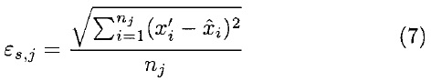
where n_j is the number of observations used in the adjustments of the multivariate regressions and j = 1,...,10, the sampling sites. The computed values are shown in Table 3. Confidence intervals of 95% were calculated using the standard error of prediction by means of the following formula:

The resulting intervals are shown in Figure 2. The observations whose values were within the confidence intervals had been considered; the percentage of success is shown in Table 3. The average success value for the monitoring sites was 96.5%, which is very close to 95%, the expected value. This agreement confirms the skill of the forecasting procedure since data for January 1997 was not included in the evaluation of coefficients, their intervention in forecasting are through, the previously mentioned, daily updating of the forecasting series.

The probability of exceeding the 0.294 ppm ozone level, P_0.294(ln(O_3,observed) > ln(0.294)) has been calculated. This value is the upper limit imposed by Mexican environmental authorities, that in case of being exceeded would lead to the launching of the environmental emergency plan. The calculations are made with the following formula:

Where Standard Norm. Dist. is the area function of the standard normal distribution. The plots of these probabilities are shown in Figure 3.

There are significant differences in the correlation coefficients for different stations. Using the data for the model fitting, corresponding to 1996, the correlation coefficients, r₂, varied from 0.45 to 0.73, while for January, 1997, the data that were used for the validation procedure, r₄ varied from 0.49 to 0.75. The most predictable values correspond to Xalostoc, San Agustin, Pedregal, Tacuba, Merced and Tlanepantla, these stations form a corridor stretching from northeast to west and then to the south. Center and southeast stations are the least predictable. This means that the factors used for forecasting explain more variability in the north and west parts of the study area. Southwest and Northwest of the MCMA show the highest ozone concentrations due to the fact that the industrial area of the city is located to the North and the pollution is transported towards the West and Southwest. The Southeast stations are located in rural and residential areas.

San Agustín, Merced, Lagunilla and Taxqueña stations probably show different patterns in the forecasting (Fig. 2) with more disperse predicted values. Taxqueña and Lagunilla stations have no information of wind speed and then the information contained in the wind was not incorporated in the model. San Agustín station has significant and high correlation coefficient between the predicted and the observed values (0.74) but only 93.5% of success in the forecasting, suggesting uncertainty in the meteorological information during the analyzed period. This observation could be extended to Merced station, which shows the same pattern.

 

5. Conclusions

The daily tropospheric ozone concentrations in the MCMA was analyzed during one-year period, it shows a non-stationary behavior and a seasonal variation can be identified, showing high values during the sunny period. This seasonal fluctuation was removed by differentiating the series once.

During 1996, the weekly variation reported by Bravo et al. (1996) was not detected, probably masked by random variations in the meteorological conditions and/or by a decrease of its magnitude due to the continuous implementation of the environmental program called one day without a vehicle. This program, which draws from circulation some vehicles during working days but allows their circulation on Saturday and Sunday, could have changed the patterns of vehicular circulation present in Bravo's study.

The historic contribution is important, as indicated by differences of correlation coefficients after the ARIMA and complete model adjustment. The exception is San Agustín station, where the history of the process is the dominant factor over the meteorological factors. The influence of the meteorological conditions occurring the same day, even a few hours before the occurrence of the ozone maximum, is a very important factor in its magnitude as demonstrated by the increase in the correlation coefficients after fitting the regressive multivariate model.

The effect of historical ozone concentrations on short term forecasting does not extend too much behind in time, this is suggested by the order of the fitted ARIMA models that do not have components of order greater than 1.

Plateros and Pedregal stations have the highest concentrations and show the greatest probability of exceeding a predetermined ozone concentration limit. These areas are not industrial, therefore the hypothesis that ozone is transported from the northeast to southwest of the valley (Bravo et ai, 1988) is reinforced.

The explained variance by the models goes from 20% to 53%. They use historic information and surrogated variables of meteorological conditions measured on the surface. The forecasting would improve significantly by adding variables containing information of the vertical structure of the atmosphere.

 

Acknowledgments

The authors want to thank the Instituto Mexicano del Petróleo for their financial support of this project, and the Red Automática de Monitoreo Atmosférico of the Departamento del Distrito Federal for making available their records. Solar radiation data were facilitated by the technical team of the Observatorio de Radiación Solar of the Instituto de Geofísica, UNAM: Ernesto Jiménez de la Cuesta, Vidal Valderrama, Rogelio Montero, Luis Galindo y Emilia Velazco. The authors also appreciate the help of O. F. Medina Mora, G. Sosa, M. G. Campos y R. Reyes, who read the manuscript and made useful suggestions.

 

REFERENCES

Böhm, M., B. McCune and T. Vandeta, 1991. Diurnal curves of tropospheric ozone in the western United States. Atmospheric Environment, 25A, 1577-1590.         [ Links ]

Bravo, H, F. Perrin, R. Sosa and R. Torres, 1988. Incremento de la contaminación atmosférica por ozono en la Zona Metropolitana de la Ciudad de México. Ingeniería Ambiental, 1, 8-14.         [ Links ]

Bravo, J. L., M. T. Diaz, C. Gay and J. Fajardo, 1996. A short term prediction model for surface ozone at southwest part of Mexico valley. Atmósfera, 9, 33-45.         [ Links ]

Bravo, J. L., M. M. Nava and A. Muhlia, 2000. Relaciones entre la magnitud del valor máximo de ozono, la radiación solar y la temperatura ambiente en la zona metropolitana de la Ciudad de México. Rev. Int. Contamin. Ambient., 16, 45-54.         [ Links ]

Box, G. E. P. and G. C. Tiao, 1975. Intervention analysis with applications to economic and environmental problems. J. Am. statist. Ass., 70, 70-74.         [ Links ]

Box, G. E. P. and G. M. Jenkins, 1976. Time Series Analysis: Forecasting and Control. Holden Day, San Francisco.         [ Links ]

Campos, M. G., P. Segura, M. H. Vargas, V. Vanda, H. Ponce, M. Selman, L. M. Montano, 1992. Ozone -Induced airway Hiperresponsiveness to noncholinergic system and other stimuli. J. Appl. Physiol., 73 (1): 354 - 361.         [ Links ]

Castañeda Pérez, L. E., 1997. Análisis por series de tiempo de las concentraciones de S02 en la ZMCM. Tesis profesional, UNAM, ENEP Acatlán, México.         [ Links ]

Chock, D. P., T. R. Terrell and S. B. Levit, 1975. Time - Series analysis of Riverside, California air quality data. Atmospheric Environment, 9, 978 - 989.         [ Links ]

Conover, W. J., 1980. Practical non Parametric Statistics, second edition, John Wiley & Sons.         [ Links ]

Cuevas, M. M., 1997. Estudio estadístico de la variación temporal de las partículas sólidas en la atmósfera de la ZMCM (PST, PM10 y Pb) Tesis profesional, UNAM, ENEP Acatlán, México, 204 pp.         [ Links ]

Draper, N. R. and H. Smith, 1981. Applied Regression Analysis, second edition, John Wiley & Sons.         [ Links ]

Finlayson-Pitts, B. J. and J. N. Pitts, 1986. Atmospheric Chemistry: Fundamentals and Experimental Techniques. John Wiley, New York.         [ Links ]

González Videgaray, M. C., 1990. Modelos de decisión con procesos estocásticos II. (Metodología de Box-Jenkins). UNAM, ENEP Acatlán, México.         [ Links ]

Instituto Mexicano del Petróleo (IMP), 1995. Sistema para el manejo estadístico de datos aerométricos de la ZMCM (SIMEDA). Programa de cómputo con Registro público de derecho de autor No. 60 523/1995. Informe técnico GCA95-13. IMP/STRP/GCA. Inédito, México D. F.         [ Links ]

Instituto Mexicano del Petróleo (IMP), 1992. Sistema Objeto Multinodal Orientado a Disco (SOMOD). Programa de cómputo con Registro público de derecho de autor No. 19366/92, México, D. F.         [ Links ]

Quadri, G. and L. R. Sánchez, 1992. La Ciudad de México y la contaminación atmosférica. Limusa, México.         [ Links ]

McColister, M. G. and K. R. Wilson, 1975. Linear stochastic models for forecasting daily maxima and hourly concentrations of air pollutants. Atmospheric Environment, 9, 417-423.         [ Links ]

Milions, A. E. and T. D. Davies, 1994a. Regression and stochastic models for air pollution - I. Review, comments and suggestions. Atmospheric Environment, 28, 2801-2810.         [ Links ]

Milions A. E. and T. D. Davies, 1994b. Regression and stochastic models for air pollution - II. Aplication of stochastic models to examine the links between ground- level smoke concentrations and temperature inversions. Atmospheric Environment, 28, 2811-2822.         [ Links ]

NRC (National Research Council), 1991. Rethinking the ozone problem in urban and regional air pollution, National Academic Press, USA.         [ Links ]

Statsoft Inc., 1994. Statistica for Windows, Statistics II. Vol III, Statsoft Inc. USA.         [ Links ]