Investigations of barotropic and baroclinic stability

 

A. WIIN-NIELSEN

The Collstrup Foundation, The Royal Danish Academy of Sciences and Letters, H.C. Andersens Blvd. 35, 1553 Copenhagen, Denmark.

 

(Manuscript received Nov. 4, 1999; accepted in final form Nov. 24, 1999)

 

RESUMEN

Mediante una expansión de funciones trigonométricas de la velocidad zonal media y de la perturbación de la función de corriente, se tratan los problemas de las estabilidades barotrópicas y de la baroclínica-barotrópica mezcladas. Se usa un modelo de dos niveles casi no divergente para manejar el problema de la estabilidad mezclada, que contienen los cizallamientos eólicos tanto vertical como horizontal en el estado básico. En la investigación presente el número de componentes en la expansión en serie se limita a cuatro, porque los perfiles eólicos meridionales más interesantes pueden ser simulados dentro de esta restricción. Los modelos se formulan en el plano beta.

El problema de los eigen valores, usando estas expansiones en serie es del tipo clásico. Pero tiene que ser resuelto numéricamente debido al tamaño de la matriz, que en el caso mezclado resulta ser una matriz de 8 por 8.

Los resultados contienen las soluciones clásicas producidas con las suposiciones dadas más simples, para ambos casos barotrópico y baroclínico, para la estabilidad máxima de ondas con una longitud de unos cuantos miles de kilómetros. Sin embargo, los modelos presentes proporcionan además inestabilidades débiles para mayores longitudes de onda para algunos perfiles del viento. Se muestra también que las corrientes básicas con dos máximos, correspondientes a los chorros subtropical y polar serán estables en el caso barotrópico, siempre y cuando este último tenga una magnitud suficientemente grande. El modo con la más grande velocidad de onda negativa para las ondas más largas es todavía una velocidad de onda comparable a la velocidad de onda de Rossby, tal como es modificada por la dimensión norte-sur del canal.

En el caso baroclínico no encontramos la misma estabilidad de los chorros dobles debido a que aún los valores medios de perfiles eólicos medios reales crearán inestabilidades para ciertas longitudes de onda.

Un análisis de la estabilidad arroja en los casos inestables la tendencia hacia un crecimiento exponencial; pero no puede manejar la interacción con el estado básico debido a los supuestos. En la última sección las ecuaciones espectrales no lineales, conteniendo las mismas componentes han sido integradas para ilustrar los desarrollos no lineales en el caso barotrópico.

 

ABSTRACT

The barotropic and the mixed barotropic-baroclinic stability problems are treated using a series expansion in trigonometric functions of the mean zonal velocity and the perturbation streamfunction. A two-level quasi-nondivergent model is used to handle the mixed stability problem, containing both horizontal and vertical wind shears in the basic state. In the present investigation the number of components in the series expansion is limited to four; because the most interesting meridional windprofiles may be simulated within this restriction. The models are formulated on the beta-plane.

The eigenvalue problem using these series expansions is of the classical type, but it has to be solved numerically due to the size of the matrix which in the mixed case becomes an 8 by 8 matrix.

The results contain the classical solutions produced with simpler assumptions giving, for both the barotropic and baroclinic case, the maximum instability for waves with a wavelength of a few thousands kilometers. However, the present models give in addition weak instabilities for much longer wavelengths for some wind profiles. It is also shown that basic currents with two maxima, corresponding to the subtropical and the polar jets, will be stable in the barotropic case provided the polar jet has a sufficiently large magnitude. The mode with the largest negative wave velocity for the longest waves is still a wave speed comparable to the Rossby wave speed as modified by the south-north dimension of the channel.

In the baroclinic case we do not find the same stability of the double jets due to the fact that even the mean values of realistic wind profiles will create instabilities for certain wavelengths.

Stability analyses give in the unstable cases the tendency for exponential growth, but cannot due to the assumptions handle the interaction with the basic state. In the last section the nonlinear spectral equations containing the same components have been integrated to illustrate the nonlinear developments in the barotropic case.

 

1. Introduction

The first investigations of atmospheric stability for synoptic and longer waves were carried out more than half a century ago by Charney (1947), Eady (1949) and Fjørtoft (1950) for the baroclinic model and by Kuo (1949) for the barotropic model. Phillips (1951) and Eliassen (1952) introduced baroclinic models with only a few information levels in the vertical direction. The results of a standard stability investigation based on the 2-level, quasi-nondivergent model are shown in Figure 1 and Figure 2, where Figure 1 gives the normal diagram showing that for a realistic vertical wind shear one obtains an interval of unstable waves with wavelength of a few thousand kilometers, while Figure 2 shows the two wave speeds in the model. In particular, it is noted from this figure that for very long waves one obtains a large negative wave speed comparable to the classical Rossby wave. Figure 3 gives an example of barotropic instability based on a simple model containing only a mean flow and a single, symmetric cosine component to describe the zonal wind and two sine-components to describe the waves (see below).

Since then a number of stability investigations have been made using a variety of models. For the barotropic case one has to make a special effort to produce simple distributions of the zonal wind where solutions for the complex wave speed may be obtained. Such examples have been produced by Kuo (1949). Eliasen (1954) used finite differences in the meridional direction to formulate the barotropic stability problem. Solutions were then obtained by numerical methods. Another approach to the barotropic stability problem was introduced by Wiin-Nielsen (1961) in which a series expansion of the perturbation streamfunction in sine-functions were selected to satisfy the boundary conditions. This approach also included the use of a similar expansion of the zonal current in cosine functions to obtain a determination of the stability and the phase speed for the case where the zonal current was described by just two components (U[0] and U[2]) giving zonal windprofiles that are symmetric around the middle of the channel. The perturbation streamfunction was also described by two components (Ψ[1] and Ψ[3]). With this limitation the equation for the eigenvalues become of the second degree and is thus easily handled. The present investigation may be considered not only as an expansion to a larger number of components, but also to the 2-level baroclinic model.

Most stability investigations are based on the filtered, quasi-nondivergent models. The stability of the waves in a non-filtered model can be expected to be different. However, a study by Wiin-Nielsen (1963), in which filtered and non-filtered models were compared, showed that the non-filtered models did have a maximum instability at somewhat smaller wavelengths than the filtered models, but otherwise the two cases are similar for wavelength of some thousands of km. In addition, it was found that very long waves are unstable for the non-filtered model with a static stability parameter increasing with decreasing pressure. For realistic values of the vertical windshear it was found that the e-folding times for the very long waves are several days indicating a relatively weak instability. The present investigation will show that ultra-long waves may also be unstable in the standard two-level model.

Frederiksen (1978) has expanded the theory of baroclinic instability to the sphere. A summary of stability investigations has been given by Hoskins (1987) with special emphasis on the low frequency phenomena.

Some expansions of the stability investigations of the barotropic model have been carried out by March et al. (1995) and Wiin-Nielsen (1995), but these barotropic studies were also limited to a consideration of wind profiles symmetric around the center of the channel, which is not typical for observed zonal wind profiles. One of the purposes of the present investigation is therefore to expand the trigonometric series to permit more general distributions of the zonally averaged state. The advantage is that realistic zonal wind profiles may be designed. The disadvantage is that the increased degrees of freedom in specifying the zonal winds are so large that it is very difficult to obtain results that may be easily classified. In the two-level baroclinic model one needs to specify 10 spectral amplitudes to describe the zonal winds, while only 5 specifications are needed for the barotropic case. It is thus impossible to investigate all cases. The strategy in the present paper is to select some interesting examples.

 

2. The barotropic model and the perturbation equations

To solve the stability problem we need to specify the zonally averaged wind U as a function of the meridional coordinate y. The perturbation equation derived from the barotropic vorticity equation may be written in the form given in (2.1) in which U(y) is the averaged zonal velocity and Ψ is the perturbation streamfunction.

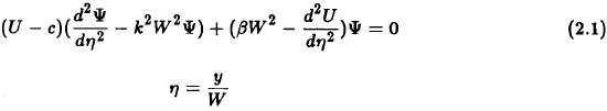
In (2.1) k = 2π/L is the wave number and L the wavelength, while W is the width of the channel. β = dƒ /dy = 1.6 10^-11 m^-1 s^-1 is considered as a constant.

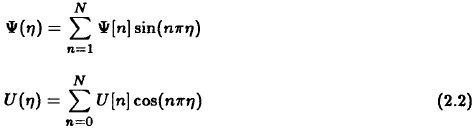
A solution of (2.1) in closed form is possible only in very special cases. In practice one may proceed either by converting the equation to a set of finite difference equations or by expanding both U and Ψ in trigonometric series. In the present study we shall prefer the latter procedure because it leads to a standard eigenvalue problem. Since the perturbation streamfunction has to vanish at the southern and northern boundaries we shall use a series expansion in sine functions.

This means that the zonal wind has to be expressed in a series of cosine functions. We use the series expansions given in (2.2).

The two series in (2.2) are inserted in (2.1). We introduce the counters q for the velocity and r for the streamfunction. To obtain the equations in wave number space we have to multiply the original equation by sin(nπη) and integrate from the southern to the northern boundary. This procedure results in an interaction integral which may be written in the form given in (2.3).

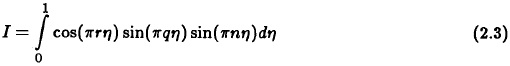
It is an elementary matter to evaluate this integral. The result is that the integral has a non-zero value only in the cases listed in (2.4). The result is obtained because a cosine function integrate to zero except when the argument is zero.

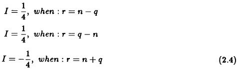
With these results we may write the general equation for component n as given in (2.5). These equations may be used for a system with any value of n. In practice, we adopt a maximum value: n_max for the description of both the zonal winds and the perturbations.

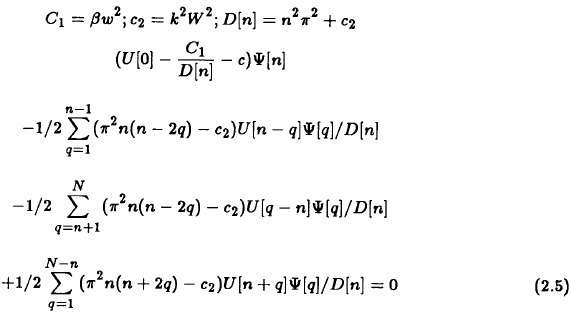
It should be pointed out that the development given above apply to the real barotropic equation. However, if the above model is changed to include a boundary condition for the vertical velocity different from zero we get an estimate of the divergence term. The net effect on the stability investigation is only that the quantity D[n] is replaced by the expression given in (2.6).

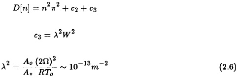
where A(p) is the function used to describe the vertical variation of the horizontal wind and A₀ = A(p₀), while A_* is the value of A at the equivalent barotropic level. We may thus easily include or exclude this effect which was introduced by Cressman (1958), using a model of a homogeneous fluid with a free surface, as a way of slowing down the ultra long waves. He determined the size of λ² empirically by running forecasts with various values and picking the one giving the best results.

The next problem is to decide on the value of N which is the total number of trigonometric components in the model. It was decided to adopt N = 4 because realistic profiles of the zonal wind may be determined by four components. Having made this decision it is a straightforward matter to determine all the terms in the 4 by 4 matrix determining the eigenvalue problem. The eigenvalues are computed from a standard numerical routine which will determine all eigenvalues as complex numbers. If the imaginary part is zero or negative we know that the component is stable. A single positive imaginary part is an indicator of instability.

 

3. Barotropic examples

A large number of examples could be produced. Each case requires the specification of the five values of U[n] for n = 0, 1,...,4 determining the variation of the zonal wind from pole to pole. Any specification provides a solution of the eigenvalue problem. A limited number of such examples will be used.

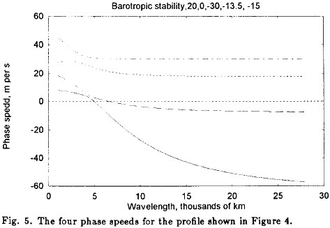
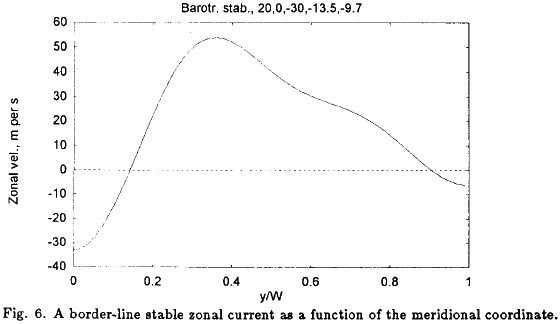
As a first example we shall present a mean zonal wind profile as seen in Figure 4. The selected values of the five coefficients are given on top of the figure. It has a subtropical jetstream and a weaker polar jetstrean with easterlies close to the southern and the northern boundaries and may be considered as a reasonable approximation to an observed profile. The solution of the eigenvalue problem shows that this profile is stable. Figure 5 shows the four phase speeds obtained from the eigenvalue solution as a function of the wavelength of the perturbation. They are all of a reasonable magnitude. We notice in particular that one of them has large negative values for large wavelength. It corresponds to the elementary Rossby solution of the barotropic equation modified by the limited width of the channel (W = 5000 km) and the wind profile. One may of course ask when the stability is replaced by instability, or, in other words, how weak can the polar jet be before instability appears, at least for some scales. The magnitude of the polar jet is to a large extend determined by the parameter U[4] which for this case is negative. The profile in Figure 6 is also stable, but if the velocity indicated by U[4] is made slightly less negative, instability appears. A polar jet of a certain magnitude is thus required to give stability.

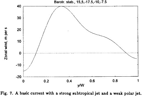
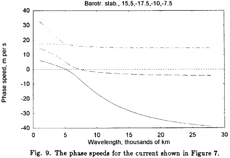
This important point is further illustrated by the next example for which the basic profile is given in Figure 7. The mean zonal wind has a strong subtropical jet with easterlies close to the southern and northern boundaries, but only a very slight indication of a polar jet. Figure 8 shows the e-folding times as a function of wavelength. We observe that instability is present from about 5000 km to the longest waves included in the calculations (28000 km). It is, however, also seen that the e-folding times for the very long waves are larger and of the order of 2 to 3 weeks thus indicating a weaker form of instability. The phase velocities for this case are displayed in Figure 9. We notice as expected that only three solutions are present from about 5000 km to 28000 km.

One may of course ask if the stability of the double jet requires a strong subtropical jet and a weaker polar jet. To answer this question the example shown in Figure 10 was designed. This profile has a strong polar jet and a weaker subtropical jet. The result of the stability calculation is that also this arrangement is stable. If we gradually reduce the magnitude of the subtropical jet in the example, we obtain eventually an unstable zonal wind profile. The profile shown in Figure 11 is still stable, but if the value of U[4] is changed from -8.6 used in Figure 11 to -8.5 we obtain instability which of course is very weak in such a border-line case. Much stronger instabilities are obtained in cases where the subtropical jet is missing. Such a profile is shown in Figure 12 with the corresponding e-folding time given in Figure 13, where the instability sets in at about 5000 km. A minimum of 1 day in the e-folding times is found at about 7000 km, while the e-folding times for the very long waves are a few days.

A general conclusion from the barotropic stability calculations is that the double jets often observed in the atmosphere constitute a stable zonal wind profile. Instability is found when one of the two maxima is reduced considerably. The cases of strongest instability is found for single jets with maxima close to the center of the channel.

Numerous other examples could be shown, but the present cases illustrate the main results.

 

4. The two-level barotropic-baroclinic problem

The model applied in this section is the standard two-level, quasi-nondivergent model where the vorticity equation has been applied at the levels of 250 and 750 hPa, while the thermodynamic equation is applied at the 500 hPa level. As usual the resulting equations have been added, subtracted and divided by 2. The result is two equations where one of them applies at 500 hPa, while the other is the thermal vorticity equation representing the layer 250-750 hPa. As in the barotropic case no forcing and no dissipation are included. The basic streamfunction for the 500 hPa level and for the thermal streamfunction are as in the barotropic case written as sums of sine-functions, while the mean zonal flows for the 500 hPa level and for the thermal layer are sums of cosine-functions. Using five components in the series for the two dependent variables, including values for the meridional averages, one obtains four spectral equations for each one of the two streamfunction given a total of eight equations for the whole model.

The derivations necessary to obtain the matrix for the determination of the eigenvalues are of the same type as in the barotropic model, but naturally a little more cumbersome due to the two equations. Most of the terms are treated the same way, but one has to be remember that the advection term in the thermodynamic equation produces two terms that have to be treated separately. From the basic equations for the two level model one obtains the following perturbation equations given in (4.1) and (4.2).

The interaction integral becomes exactly the same as in the barotropic case, see equation (2.2). Based on (4.1) and (4.2) it is then possible to derive the eight perturbation equations whose coefficients determine the matrix of the eigenvalue problem. The dimension of the matrix is 8x8 in the baroclinic case. The same computer program as in the barotropic case is used to calculate the eigenvalues.

 

5. Barotropic-baroclinic examples

It should be stressed from the very beginning of this case that a distinct difference should exist between the barotropic and the baroclinic cases. A constant wind U in the barotropic case gives only stable solutions, while constant winds U_*[0] and U_T[0] will create instability in the baroclinic case if U_T[0] is sufficiently large.

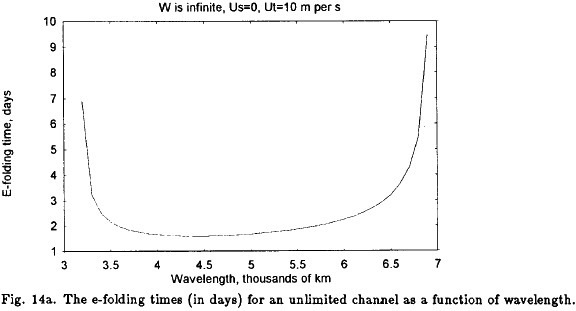
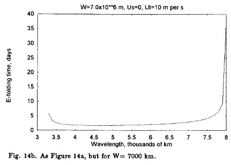
We shall first illustrate the effect of the width of the channel. In the classical investigations of stability based on the two-level, quasi-nondivergent model it is assumed that the channel is infinitely wide. The e-folding times are shown in Figure 14a. Setting the width of the channel to 7000 km.and repeating the analysis of stability we find the e- folding times shown in Figure 14b. The minimal e- folding time has become slightly larger and the wavelength interval in which we find instability has in the upper limit expanded from 7000 km to 8000 km. In Figure 14c the width of the channel has been decreased to 3500 km with the result that the region of instability has increased to an upper limit of 28000 km. It should be recalled that although a width of 3500 km is small, it will appear in the present model as wave number 2 in the description of the zonal wind and the perturbation stream-function, if the total width of the channel is 7000 km. The smaller scales are necessary to give realistic profiles of the zonal winds, and it may thus be expected that instability will be found at larger wavelengths than in the simple case permitting only constant zonal winds.

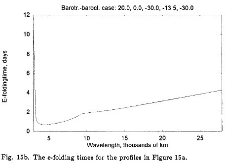
A first question to answer is whether or not the stable case of a double jet found in the barotropic case has a counterpart in the baroclinic case. From the simple stability analysis in which U_*[0]and U_T[0] are constants we are used to think that the only parameter of importance for stability or instability is the magnitude of U_T. For a sufficiently large value of U_Twe will find an interval in which the waves are unstable. The question is therefore if the changes of U_* and U_Twith respect to the south-north coordinate, i.e. the barotropic effect, is sufficiently large to create a stable case. To investigate this question an example has been constructed, see Figure 15a. It has the values of U_* as shown in the title of the figure. The values of U_Tare half of the values for U_*. In general we have for the winds at the surface that U_s = U_* — 2U_T, but U_s is of course zero in the present example. The profiles shown in Figure 15a are unstable for the interval shown in Figure 15b. For each wavelength the real and the imaginary values of the wave speed have been sorted with respect to size. Figure 15b contains only the largest values of the imaginary part of the wave speed and thus the smallest values of the e-folding time, i.e. the most unstable mode. We notice small e-folding times of the order of 1 day for a wavelength of about 5000 km. At wavelengths a little smaller than 10000 km we notice a small discontinuity indicating that the smallest values of the e-folding times come from another mode. The e-folding time is slightly larger than 4 days for the longest waves. We can therefore conclude that the double jet under investigation is unstable in contrast to the barotropic case.

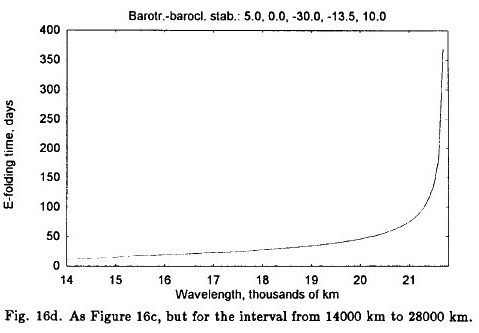
In the next example we consider a zonal flow with a single maximum as seen on Figure 16a. The westerly jet is surrounded by easterlies to the south and to the north. The instability comes in three parts. Very short waves are unstable in a small interval from 1500 to 2200 km in wavelength. The e-folding times are moderately large with a minimum at about 3 days, see Figure 16b. A separate region of instability is found from 3200 km to almost 22000 km.

It is shown in two parts. Figure 16c goes to 14000 km and indicates a maximum instability around 4000 km, where the e-folding time is 1 day. A secondary minimum is found between 9000 and 10000 km with e-folding times of a little less than 3 days, whereafter the e-folding times continues to increase as can be seen on Figure 16d. This figure shows that the instability becomes extremely weak.

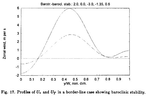
It is of interest to determine how weak the zonal winds have to be in the baroclinic case to obtain stability for all wavelengths. Depending on the shape of the profiles of the zonal winds there are probably many answers to this question. A single example will be shown. The present example started from the profiles with double jets shown in Figure 15a. All values of U_*[n] and U_T[n] were divided by 10 except for U_*[4] and U_T[4] which were set to -2 and -1, respectively. It turns out that the resulting profiles of the zonal winds are stable for all wave lengths. The two values of U_*[4]and U_T[4]were gradually increased to 0.7 and 0.35 where instabilities start to appear. The borderline case of the zonal profiles with the values at U_*[4]= 0.6 and U_T[4] = 0.3 is shown in Figure 17. The stability analysis shows that these profiles are stable for all wavelengths.

 

6. Integration of the corresponding nonlinear barotropic equations

The purpose of this section is to show in the barotropic case the results of some integrations of the nonlinear spectral equations containing the same components as in the barotropic stability analysis. The wave components were complex quantities in the stability analysis. For the purpose of integrating the nonlinear equations it is an advantage to divide each of the equations in the real and the imaginary parts. In addition, it is necessary to formulate the equations for the rate of change of the four components of the zonal wind. The latter is most easily done by using the first equation of motion which for the barotropic case reduces to the very simple equation given in (6.1).

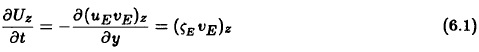
The subscript E refers to eddy components, while the subscript z indicates the zonal average. We have further made use of the fact that for nondivergent motion the divergence of the eddy momentum transport is equal to the eddy vorticity transport. When the specification of the eight eddy components of the streamfunction is introduced in (6.1) together with the four time-dependent components of zonally averaged wind it is possible to derive the equations for the rate of change of the four amplitudes of the zonally averaged wind. In the real domain we have thus a nonlinear, low-order model consisting of 12 coupled equations. These equations can be integrated numerically as an initial value problem. Heun's scheme has been used for the time integration.

The system of equations shall of course be able to reproduce the results of the stability analysis if the initial values of the streamfunction components are selected to be very small, while the initial values of the four zonal wind components should be identical to those for which the stability analysis has been made. As a check on the correctness of the derivations we recall that the total kinetic energy is conserved in the barotropic case without forcing and dissipation. The sum of the zonal and eddy kinetic energies should thus, also for the system truncated to four components for each real variable, be equal to the initial kinetic energy. The system as formulated conserves the total kinetic energy with a good accuracy. A full constancy cannot be expected due to the finite differences used in the time integrations.

As a first case the stability of the double jet was tested by integrations of the 12 equations. A complete agreement was found with the earlier results including also the border-line profile representing the change from stability to instability.

In the remaining examples the initial zonal wind profile is given by the values: U[1] = 0.0, U[2] = -30.0, U3 = -13.5 and U[4] = 5.0, all in m per s. The initial values of all the components of the eddy streamfunction were 1.0 x 10⁵ m² s^-1 or small deviations from this value as specified later. The wavelength was 5000 km and the width 7000 km. The time step is 15 minutes in all cases.

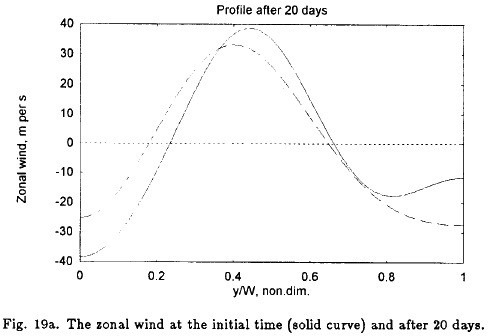
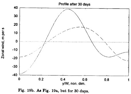
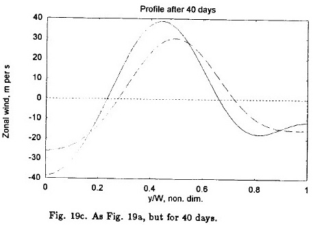
Figures 18a, 18b and 18c show the streamfunction at 5, 10 and 15 days indicating that a travelling wave has been generated. The wave will interact with the zonal flow. Figures 19a, 19b and 19c contain the initial zonal wind profile as the solid curve, while the dashed curves show the zonal wind profiles at 20, 30 and 40 days indicating that the position of the maximum zonal wind will oscillate around the maximum of the initial wind profile as energy exchanges take place between the zonal kinetic and the eddy kinetic energies.

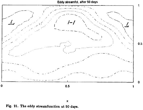
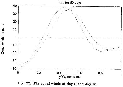
The integration was carried out to 100 days. Figure 20 shows the zonal kinetic energy (solid line) and the eddy kinetic energy (dashed line), while the dotted line gives the total kinetic energy. It is seen that the numerical integration conserves the total energy. The maximum eddy kinetic energy is found around 50 days. The eddy streamfunction for this time is displayed in Figure 21, while Figure 22 shows the initial zonal wind profile (solid curve) and the same profile at 50 days. The eddies to not disappear entirely at minimum, which can be seen from Figure 23 showing the eddy kinetic energy as a function of time for 200 days. We have thus demonstrated that quasi-periodic motion is present in the barotropic model with a very large time scale which in the present example is about 100 days, starting with a very small initial amplitude of the eddy streamfunction.

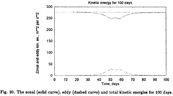
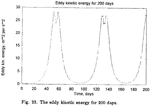
One may get the impression that there is a discrepancy between Figures 18 and 19 describing the development for relatively short times and Figure 20 covering 100 days. The apparent discrepancy is entirely due to the production of the figures. When Figure 20 is plotted for the first 20 days one has a clear indication of the phenomena described in Figures 18 and 19 indicating the repeated creation of waves with a much shorter lifetime than the quasi-period time scale of about 100 days.

 

7. Conclusions

The formulation of the barotropic and baroclinic stability problems treated in the investigations are more general than those employed in earlier treatments. The use of spectral components permits the specification of quite general basic windprofiles.

A main result for the barotropic case is that the stability analysis of double jets corresponding to the subtropical and polar wind maxima shows stability for all wavelengths. The stability is changed to instability for some wavelengths when one of the maxima is decreased in size relative to the other. Strong instabilities are found for zonal winds with only one maximum.

The result quoted above for the barotropic case is not valid for the baroclinic case for realistic specifications of the zonal winds. The reason is that a realistic zonal wind profile contains sufficiently large values of U_T[0] to create instabilities. It is, however, demonstrated that for low values of UT[0] one will find stability.

Another main result is that the region of instability in wavelength space for the present formulation is extended to the very long waves in some cases. The wavelengths for which instability is found are often divided in two separate regions. However, the rate of instability as measured by the e-folding times indicate that the instability for very long waves in general is much weaker than for the shorter waves and dominated by e-folding times as large as 1 to 3 weeks.

A nonlinear model with the same components as in the perturbation analysis has been designed. It contains 12 real components with 4 components to describe the zonal flow and 8 components for the eddy streamfunction. An example starting from a given zonal wind profile and very small amplitudes on all eddy components shows quasi-periodic motion with a time scale of about 100 days during which the eddy amplitudes go from a minimum to a maximum value in about 50 days, whereafter the eddies decrease in intensity to a small value.

 

Appendix

 

REFERENCES

Charney, J. G., 1947. The dynamics of long waves in a baroclinic westerly current, Jour. of Meteor., 4, 135-162.         [ Links ]

Cressman, G. P., 1958. Barotropic divergence and very long atmospheric waves, Mo. Wea. Rev., 86, 245-250.         [ Links ]

Eady, E.T., 1949. Long waves and cyclone waves, Tellus, 1 (3), 35-52.         [ Links ]

Eliasen, E., 1954. Numerical solutions of the perturbation equation for linear flow, Tellus, 6, 183-191.         [ Links ]

Eliassen, A., 1952. Simplified models of the atmosphere, designed for the purpose of numerical weather prediction, Tellus, 4, 145-156.         [ Links ]

Fjørtoft, R., 1950. Applications of integral theorems in deriving criteria of stability for laminar flows and for the baroclinic circular vortex, Geof. Publ., 17, 52 pp.         [ Links ]

Frederiksen, J. S., 1978. Growth rates and phase speeds of baroclinic waves in multi-level models on the sphere, Jour. Atmos. Set., 35, 1816-1826.         [ Links ]

Hoskins, B. J., 1987. Low-frequency dynamics - Linear theory, Dynamics of low-frequency phenomena in the atmosphere, Vol. 2, Nat. Center of Atm. Res., 317-398.

Kuo, H. -L., 1949. Dynamic instability of two-dimensional nondivergent flow in a barotropic atmosphere, Jour. of Meteor., 6, 105-122.         [ Links ]

March, N. D., I. A. Mogensen and A. Wiin-Nielsen, 1995. On free and forced barotropic flows and their stability, Geophysica, 31(2), 47-57.         [ Links ]

Phillips, N. A., 1951. A simple three-dimensional model for the study of large-scale extratropical flow patterns, Jour. of Meteor., 8, 381-394.         [ Links ]

Wiin-Nielsen, A., 1961. On short-and long-term variations in quasi-barotropic flow, Mo. Wea. Rev., 89, 461-476.         [ Links ]

Wiin-Nielsen, A., 1963. On baroclinic instability in filtered and non-filtered numerical prediction models, Tellus, 15, 1-19.         [ Links ]

Wiin-Nielsen, A., 1995. On stability of jet streams, Atmósfera, 8, 143-155.         [ Links ]