The zonal atmospheric structure: A heuristic theory, Part III

 

A. WIIN-NIELSEN

The Collstrup Foundation Royal Danish Academy for the Sciences and Letters H.C. Andersens Blvd. S5, 155S Copenhagen, Denmark.

 

(Manuscript received Aug. 18, 1999; accepted in final form Sept. 13, 1999)

 

RESUMEN

Se diseña un modelo de la estructura zonalmente promediada de la atmósfera. Se emplean coeficientes de intercambio para describir los transportes meridionales de las propiedades cuasiconservativas. Al contrario de los modelos previos, los coeficientes de intercambio tienen una variación meridional especificada que sustituyen a los coeficientes constantes usados en los estudios anteriores. El modelo básico es un modelo cuasi-geostrófico de dos niveles. El tiempo de integración de las ecuaciones del modelo es llevado al cabo en el dominio espectral, empleando las ecuaciones esféricas. El truncamiento de los polinomios de Legendre en el modelo es n = 10, pero puede elegirse libremente.

Mediante la simetría alrededor del Ecuador el calentamiento de la atmósfera se prescribe con base en los estudios observacionales. Las integraciones permiten una determinación de la variación meridional de la temperatura resultante, los geopotenciales de los vientos zonales en los niveles superior e inferior; asimismo de los transportes de calor sensible para el modelo atmosférico y la velocidad vertical, además de los transportes de momento en los niveles superior e inferior. Las relaciones de energía del modelo pueden también ser determinadas.

Los resultados están razonablemente de acuerdo con la estructura zonal observada de la atmósfera.

 

ABSTRACT

A model of the zonally averaged structure of the atmosphere is designed. It employs exchange coefficients to describe the meridional transports of quasi-conservative quantities. In contrast to earlier models the exchange coefficients have a specified meridional variation replacing the constant coefficients used in previous studies. The basic model is the two-level, quasi-geostrophic model. The time integration of the model equations is carried out in the spectral domain using the spherical equations. The cut-off for the Legendre polynomials in the model is n=10, but can be selected freely.

Employing symmetry around the equator the heating of the atmosphere is prescribed based on observational studies. The integrations permit a determination of the meridional variation of the resulting temperature, the geopotentials, the zonal winds at the upper and the lower levels, the transports of sensible heat for the model atmosphere, the vertical velocity and the transports of momentum at the upper and the lower levels. The energetics of the model may also be determined.

The results are in reasonable agreement with the observed zonal structure of the atmosphere.

 

1. Introduction

The previous two papers on the present subject (Wiin-Nielsen, 1994 and 1999) have considered the zonal atmospheric structure in a two-level quasi-geostrophic model and a model consisting of a homogeneous fluid with a free surface. In the zonal models the atmospheric eddies are parameterized by constant exchange coefficients. The purpose of the present paper is to use the two-level quasi-geostrophic model once more, but with exchange coefficients with a prescribed meridional variation. The reader is referred to the first two papers in this series for a general introduction to the subject.

The general principles for the parameterization of the transports can be expressed by assuming that the meridional transport of a quasi-conservative quantity may be expressed using an exchange coefficient. If Q is a conserved quantity in adiabatic and frictionless flow then the parameterization of the meridional transport of Q can be expressed as follows:

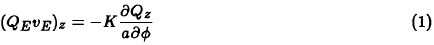
In the formula a is the radius of the Earth and the derivative is with respect to latitude. The coefficient K has the dimension m² s⁻¹ , and it can in principle be a function of pressure and latitude. The quasi-conservative quantities in quasi-nondivergent models are the potential vorticity and the potential temperature.

The author (Wiin-Nielsen, 1994, 1999) has investigated these ideas in two cases. In the first case the exchange coefficients were constants. In the two level, quasi-geostrophic model the conserved quantities in the non-forced case is the potential vorticity at the upper and lower level and the potential temperature at the middle level. Using these principles on an even simpler model, i.e. a forced homogeneous fluid with a free surface, it was possible to obtain a qualitatively correct meridional distribution of the zonal winds using constant exchange coefficients (Wiin-Nielsen, 1999).

The exchange coefficients are functions of latitude with a maximum in the latitudinal band dominated by wave generations due to barotropic and baroclinic processes and minima at the high and low latitudes. It is likely that the maximum value of the exchange coefficient will vary with the position of the largest barotropic and baroclinic wave activity, but so far it has not been possible to define the values of the exchange coefficients in this way. We shall therefore define the latitudinal variation of the exchange coefficients by giving them a fixed mathematical form as a function of latitude.

The purpose of the paper is thus to use the two-level, quasi-geostrophic model with variable exchange coefficient to determine the distribution of the temperatures, the geopotentials and the zonal winds with latitude. In addition, we shall use the parameterizations to make indirect calculations of the vertical velocity, the transports of sensible heat at the middle level and of momentum at the upper and the lower levels. The model will also be used to determine the zonal energetics of the model.

 

2. The model

The basic principles of the model has been discussed in earlier papers (Wiin-Nielsen, 1994, 1999). It is thus sufficient to state that the two basic equations are derived by using the two-level, quasi-geostrophic model recalling that the parameters entering the equations are all zonally averaged quantities. As usual the equations applying at level 1 (250 hPa) and at level 3 (750 hPa) have been added and subtracted to give equations applicable at the middle level (500 hPa) and for the thermal flow corresponding to a layer of 250 hPa. The heating has been introduced as an unspecified quantity to be taken from studies based on observations. The dissipation has been introduced partly as dissipation at the surface of the Earth, i.e. at level 4 (1000 hPa) and partly as internal friction depending on the vertical windshear (Charney, 1959). The parameterization of the meridional transports of the potential vorticity and of sensible heat have been introduced in the following two equations, (2.1) and (2.2).

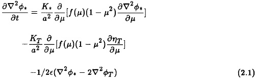
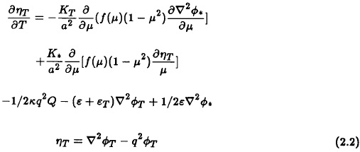
ƒ(μ) is the function specifying the variation of the exchange coefficients with latitude with the definition that μ = sin(φ). The coefficient is then of the form Kƒ(μ). The function ƒ(μ)is in all cases of the paper defined by

This specification results in vanishing values at equator and pole with a maximum for μ = 2^−½ corresponding to 45 degrees. The definition in (2.3) was selected because it is the most simple function that is symmetric around the equator and that vanishes at μ = 0 and at μ = 1. The specification is in qualitative agreement with the exchange coefficients determined from observations, but while the small values of the exchange coefficients in the low latitudes seem to be justified it is less certain that the values close to the pole are completely realistic.

The equations (2.1) and (2.2) are integrated with respect to time hopefully going to an asymptotic steady state. In the present case we shall use the spectral method, because relatively few spectral components are sufficient for our purpose. The problem is thus to bring the basic equations (2.1) and (2.2) with the specification in (2.3) into the spectral domain. To do this one has to use a number of the formulas valid for the Legendre polynomials, since we have to express non-trivial terms involving the Legendre polynomials in sums and differences of these functions.

The most important formulas of this kind are given below.

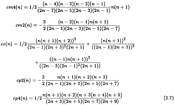
Using the first of the formulas given above we find that the Legendre polynomials will involve P_n+1 and P_n−1 and the corresponding values P_q+1 and P_q−1 where n and q are the two counters. The multiplier μ on each term gives formulas involving P_n+2 P_n and P_n−2 with the corresponding Legendre polynomials in the counter q. Using next the orthogonality of the Legendre polynomials and applying the normal procedure for the derivation of the spectral form of the equations we find after some algebraic work that any of the differential terms in (2.1) or (2.2) for a wave number n as expected will involve the Legendre polynomials with wave numbers (n −4), (n−2), n, (n + 2) and (n + 4). The major steps in these derivations are given in Appendix 1. Any of these terms will be converted to an expression of the type given in (2.6) where the variable is denoted by L.

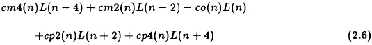
The expressions for the coefficients are given in (2.7). These expressions are general, and they may be calculated for arbitrary values of n. The coefficient cm4(n) will be non-zero only for n > 4 just as cm2(n) is non-zero only for n > 2. Similarly, the coefficients cp2(n) and cp4(n) should be disregarded for n = n_max or larger values.

After these derivations it is sufficient to decide on the wave numbers that will be included in the integrations. The results given in the next section are all obtained for n_max = 10. For this wave number the Legendre polynomial has 5 zeroes between equator and pole. The choice of n_max is thus sufficient to describe the expected distributions if the model is schematically correct. The selection of the maximum number of components in the model has an influence on the results. If n_max is too small the results will not be representative for the observed atmosphere. A values much larger than 10 of n_max results also in unrealistic results. This is due to the fact that the parameterizations contain terms that generate vorticity as well as terms with the opposite effect as can be seen from equations (2.1) and (2.2).

In the selected case with n_max = 10 we get a system of 10 equations, 5 of them are related to the middle level (about 500 hPa) while the remaining 5 equations describe the thermal flow. These equations are integrated in time, and it turns out that the model approaches a steady state after integrations over about 200 days.

The steady state solution is then used to calculated the components of the zonal winds at the upper and the lower levels. This is done by using the balance equation for the components. Thereafter one obtains the wind distributions by evaluation of the sum of the series expansion in Legendre polynomials.

The meridional transports of sensible heat for the atmosphere and the momentum transports at the upper and lower levels are also obtainable from formulas given in the previous papers (Wiin-Nielsen, 1994, 1999).

 

3. The results

To test the model we have used the averaged heating of a single winter month from the global analyses of the European Centre for Medium-Range Weather Forecasts. Based on the gridpoint data for the zonally averaged heating the coefficients of the expansion in Legendre polynomials were obtained. All coefficients for odd numbers of the Legendre polynomials were disregarded to obtain a heating distribution symmetric around the equator. The coefficients for the even components up to and including n_max were used in the integrations for 200 days.

Figure 1 shows the heating distribution from equator (q = 0) to the North Pole (q = 100). To obtain the latitude from this and the other figures we note that the latitude is arcsin(q/100). As examples we find that q = 50 corresponds to a latitude of 30 degrees, while q = 70 is close to 45 degrees of latitude.

The temperature distribution is given in Figure 2. It shows that the total temperature difference between equator and pole is about 30 degrees K which is of a reasonable order of magnitude for the winter season. The geopotentials for the vertical mean flow (solid curve) and the thermal flow (dashed curve) are displayed in Figure 3. The model produces a larger variation in the geopotential of the mean flow than of the thermal flow in agreement with the structure of the real atmosphere.

To obtain the distribution of the zonal winds (uz) at the two levels it is necessary to use the balance equation expressed in wave number space to obtain the Legendre coefficients for the vorticity from the corresponding numbers for the Laplacian of the geopotential. As remarked in Wiin-Nielsen (1999) it is necessary to assume either that the coefficient of the vorticity for wave number 1 is zero or to compute it from the second components of the heating. The latter procedure has been used in the present example. From the coefficients for the vorticity we obtain the corresponding values for the stream-function. These numbers are then used to calculate the zonal winds at the required levels. They are seen in Figure 4. The winds are stronger at the upper level than at the lower level. A maximum wind speed of about 50 m per s is seen in the subtropical jet located at about 25 degrees of latitude. A polar jet located around 62 degrees of latitude has a maximum of about 30 m per s. We observe also easterlies in the low latitudes and weak easterlies close to the pole. The winds at the lower level are much weaker with maxima in about the same location as at the upper level. Figure 5 gives the zonally averaged winds at level 4 (1000 hPa). Also these winds seem to have a reasonable magnitude.

The estimate of the total transport of sensible heat as computed from the parameterization is shown in Figure 6. Note that the numbers are divided by 10⁷ to create a better figure. The maximum heat transport is located close to 45 degrees with a value that is of the correct order of magnitude for the winter season as can be seen by a comparison with the heat transport for December, January and February as given (on page 66) by Wiin-Nielsen and Chen (1993). The quantity given in Figure 6 is H_T = c_p p₀ (Tv)_z/g, while the observational study gives (Tv)_z. Using approximative values we find that c_p p₀/g = 10⁷. The two figures are therefore comparable. Figure 7 shows the momentum transport as calculated from the parameterization of the transport of the potential vorticity at the two levels. The basic formula is given in Wiin-Nielsen (1999). Figure 7 shows that the transport is larger at the upper than at the lower level. The maximum northward transport is located slightly to the south of 30 degrees, while the maximum southward transport is found at about 55 degrees of latitude. The magnitude of the momentum transport at the upper level computed from the model is of the same order of magnitude as the transport computed from observation for the winter months (Wiin-Nielsen and Chen, 1993).

Figure 8 shows the zonally averaged vertical p-velocity as computed from the steady state thermodynamic equation. The figure indicates a Hadley type cell with rising motion at the equator and the largest sinking motion at q=35 (about 20 deg. N). Rising motion takes place north of 30 deg. N to 75 deg. N, while weak sinking motion is found over the polar region. The motion is weak with a maximum that is about 0.5 mm per s.

The heating employed in the above example was computed from analyses and thus based on observations. However, it is not necessary to have heating on all the even components to obtain similar profiles. If we include the heating on component 2 only, in which case the distribution of the heating is determined by the second Legendre polynomial, and repeat the integration we obtain results with similar distributions of all the parameters. The reason for this behavior is that the second component dominate in the distribution of the diabatic heating, and that the steady state values for the other parameters will have non-zero values on all components included in the integration.

The energetics of the present case may be calculated using the standard formulas for the two-level model. It is found that A_z = 5452kJm⁻², K_z = 3700kJm⁻², G(A_Z) = 4.81Wm⁻², C(A_Z, A_e) = 5.12Wm⁻², C(A_z,K_z) = -0.31Wm^-2, C(K_e,K_z) = 1.90Wm⁻² and D(K_z) = 1.59 Wm⁻². These values have the correct directions and a reasonable order of magnitude.

 

4. Concluding remarks

The present version of the zonally averaged model with its parameterization of the transport processes using exchange coefficients with a prescribed variation in the meridional direction gives results that are superior to those obtained from earlier versions of the model. The improvements are due to the exchange coefficients since all other processes have been treated in the same way as in previous models. The results may be taken as an indication that the parameterizations of the eddy transports of quasi- conservative quantities employed in the present model are better than the models with constant exchange coefficients. The numerical values of K_* and K_T were determined in such a way that the average over all latitudes is equal to the constant values employed earlier and based on observational studies.

 

Appendix 1

 

REFERENCES

Charney, J. G., 1959. On the general circulation of the atmosphere, The Atmosphere and the Sea in Motion (Rossby Memorial Volume), 178-193.         [ Links ]

Wiin-Nielsen, A., 1994. The zonal atmospheric structure: A heuristic theory, Atmósfera, 7, 185-210.         [ Links ]

Wiin-Nielsen, A., 1999. The zonal atmospheric structure: A heuristic theory, Part II, Atmósfera, 12, 189-198.         [ Links ]

Wiin-Nielsen, A. and T.-C. Chen, 1993. Fundamentals of atmospheric energetics, Oxford University Press, 376 pp.         [ Links ]