nueva página del texto (beta)
 Inglés (pdf)
 Artículo en XML
 Referencias del artículo
 Enviar artículo por email
 Citado por SciELO
  Similares en
SciELO
Similares en
SciELO 
 Permalink
1. Introduction
Discussion about which is the greatest, strongest, biggest, and most accomplished team in Mexican football (known as soccer in Australia, Canada, the United Kingdom, United States, among many others) is frequent in Mexican media. Most of the time, the discussion is mainly driven by preconceived ideas, feelings, or other idiosyncrasies of football commentators. In this way, the conclusions that usually arise are, more often than not, based on a shallow appreciation of the statistics concerning Liga MX (Professional Football Mexican League, First Division), considering only the historical titles or recent titles, the popularity among fans or the media time covered by journalists, so that conclusions reached in the media are based on a trivial analysis of a small number of variables.1 Consequently, sports commentators will pay asymmetrical attention to sporty measures as the number of domestic and international titles, number of play-offs, recent competitive performance, and some non-sporty indicators like the number of fans, media factor and the market value of the franchises. Hence, the opinion of sport commentators tends to be diffuse, as it lacks a statistical measure that incorporates the several elements that allows to conclude which team is the greatest in Liga MX. Our research pretends to fill this gap.
Dominance is rather stable in European leagues. Indeed, it is not uncommon to see major teams constantly championing their tournaments. For example, Real Madrid C.F. and F.C. Barcelona rule the Spanish league, while Manchester United F.C., Chelsea F.C., Liverpool F.C. and Manchester City F.C. often win England’s national tournament. On the contrary, in Mexico, such a dominant team does not exist, and popularity is not a simple matter either. The champion has changed so much that expressions such as “in Liga MX just about anything can happen” is a well-known motto, particularly during play-offs and under the short championship’s era. Thus, our research question arises in the context of a changing structure of the tournaments through time and is not directly adaptable to reflect the Elo-like FIFA point-awarding scheme. Under this system, one may argue that the strongest team would be the one with the highest points reached in the league; however, this criterion may not accurately reflect the Liga MX-specific characteristics. Popularity, understood in this article as people’s like, is often taken to be the reflection of a team’s strength by assuming that people follow a particular team on feelings and historical competitive sports performance. Nevertheless, Liga MX is also complicated in this respect. Some analysts suggest that C.D. Guadalajara is the most followed team, its popularity stemming from the fact that all its players are Mexican and its dominance in the 1960s. However, others argue that it is Club América who gains the most public attraction due to the number of titles, the high media presence, the large number of foreign players in its roster and for the national football rivalry with Guadalajara. Other teams are C.F. Cruz Azul, who dominated the Liga MX during the 1970s, and Club Universidad Nacional (hereafter, UNAM), the team of Mexico’s largest and most important public university. In this way, it is very common that in sports media TV, football analysts refer to these four teams as “the four biggest”.2
Recently the “northern teams” such as Club Tigres de la Universidad Autónoma de Nuevo (hereafter, UANL), C.F. Monterrey, Club Santos Laguna, and Club Tijuana have gained importance mainly due to the economic investment in the last years. In this context, UANL is known as the “team of the decade”, having obtained five titles since 2010. Thus, just as rankings and dominance, popularity cannot be seen as a unique, reliable measure of a team’s greatness in Liga MX.
This paper is related to literature that studies the team’s rankings from an econometric and statistical viewpoint. For example, Maher (1982) considers the team’s offensive and defensive strengths and weaknesses as parameters of the home and away team’s independent Poisson-distributed goal scoring. He considers a hierarchy of models and finds that bivariate models that consider the dependence between the scores of the two teams improve the fit considerably. Although this method offers a measure of dominance that helps determine the best and strongest team in England, it is only based on the number of goals scored in successive matches. Such a consistent approach for identifying the strongest team in the league is, of course, not expected of sports commentators. Nonetheless, a more quantitative approach to ranking a team’s performance is, in many respects, desirable.
Glickman and Stern (1998) treat a team’s strengths as latent, time-varying factors which serve as inputs in a predictive model for game scores. Stefani and Pollard (2007) review some of the most widely ranking systems in different football codes, although much of the methodology used in these systems is not statistically oriented.
The most widely known and used ranking system for association football is the FIFA/Coca-Cola World Ranking. This system was recently modified and resembles now chess’ Elo system, where the difference in the ratings between two individual players serves as a predictor of a match’s outcome; thus, the team’s rating is computed in an additive, accumulative manner. Mikolajec et al. (2013) analyze 52 performance variables for the National Basketball Association (NBA) teams to conclude that primarily offensive factors determine sports performance. Also, Baker and McHale (2015) use a dynamic model to estimate the strengths of football teams based on historical sports results, and Corona et al. (2017) modify the FIFA rating using other covariates to predict 2014 FIFA World Cup and 2015 Copa América. Another interesting analysis is carried out by Georgievski et al. (2019), who use English Premier League data to investigate what influences the success of football teams by applying factor analysis and a panel data approach. Their main results suggest that it is more important for bottom-ranking teams to play better defensively than offensively. In contrast, for top-performing teams, the probability of success is more affected by the offensive style. Similarly, Georgievski and Labadze (2020) use the Balassa index, which measures the revealed comparative advantage, to examine how basketball has changed in the last 10 years, which part of the game has become more important, and how stronger teams compare to weaker teams.
Recent research applied for Liga MX is developed by Corona et al. (2021) who use Dynamic Factor Models (DFM) to estimate the common factors with percentage of points reached of the teams in the short tournaments. They conclude that the first common factor is stationary, dominated by teams such as América, Guadalajara and Cruz Azul. The second common factor is non-stationary and highlight teams as UANL, Monterrey and Club de Fútbol Pachuca. Also, Velázquez-Guadarrama and Hernández-Velázquez (2022) estimate the effect of a change of coach during mid-term in the competition, concluding that the change does not improve the teams’ performance. However, we take a longer-term approach to assess the dominance in the league since its inception.
The main difference of this work with respect to previous literature is that we do not use only sporty variables to analyze themes related to sports analytics/economics, specifically in this case, to define the “greatness” in Mexican football. Therefore, we consider club performance variables like the total number of championships won, the total number of games played in regular seasons, and so on. Nevertheless, we also consider non-sporty related variables, such as popularity, which are computed as a percentage share in a survey taken at the beginning of the regular season by Mitofsky,3 and each team’s attendance in their stadiums. Additionally, we consider the market value of the franchises’ roster. Hence, “greatness”, being a multidimensional concept, ought to take all these variables into account to construct such a statistical indicator and their interrelations. For these reasons, we use a multivariate statistics technique, Principal Component Analysis (PCA), to derive a statistical indicator that can factor several interdependent ones without making distributional assumptions, thus being more robust than, for example, likelihood-based methods. We apply PCA recurrently at each end-of-season from Apertura 2011 to Apertura 2019,4 which allow us to analyze the statistical significance of the variables on the factor loadings and the estimated scores and study their evolution over time.
Consequently, the main contribution is to provide an econometric/statistical approach to generate an indicator that helps answer a frequently asked question by the Mexican sports media: Who is the greatest team in Liga MX? Hence, we disentangle the most relevant variables in the “greatness” concept and evaluate the statistical significance of the variables and the econometric indicator.
The rest of the paper is organized as follows. Section 2 summarizes the components’ estimation and loadings using PCA, discusses the selected variables and their construction, and shows a descriptive analysis. Section 3 presents a brief explanatory analysis. Section 4 describes the results of the methods, and section 5 concludes and comments the further research.
2. Methods and data
2.1 Principal components analysis
The estimation of the principal components, latent variables or factors is carried out through PCA. Although one of the main goals of PCA in many applications is reducing dimensionality, we chose this technique because it highlights the most notable directions of variation in a given set of variables. As is well known, given a matrix X of dimensions N × K, where N is the number of items and K is the number of variables, the first principal component solves the maximization problem:
Thus, the matrix P (factor loadings) produces the linear
combination
2.2 Determining the number of components
In practice, the number of components of factors, r, must be
estimated. The most common criterion to determine r is related
with the percentage of variance explained by the r-th principal
component estimated as
This criterion is given by
where
We determine
2.3 Data
The variables that we use capture measures of the teams’ competitiveness, popularity, and financial health. Particularly, we consider the following dataset:
Domestic tournaments5
Titles: Number of titles in Fist Division (accumulated since 1943 to Apertura 2019). It indicates the dominance in domestic tournaments during the professional stage.
GP: Games played in the regular season (accumulated since 1943 to Apertura 2019).
Points: Points per match in regular season (accumulated since 1943 to Apertura 2019). It indicates the performance of the teams in regular season.
GP-P: Games played in play-offs (accumulated since 1970 to Apertura 2019). It shows the presence in the “Liguilla” stage implemented since 1970, the championship’s tournament played
by the qualified teams.
Copa MX: Number of titles in Copa MX (accumulated from 1942 to 2019). Provides information about the team’s dominance in the alternative and domestic tournaments.6
International tournaments7
CONCACAF: Number of titles in the Confederation of North, Central America, and Caribbean Association Football (CONCACAF) Champions grpLeague (accumulated from 1968 to 2019). It
shows the dominance of the Mexican teams in the CONCACAF area.8
GP-CONMEBOL: Games played in the South American Soccer Confederation (CONMEBOL). It includes Copa Libertadores (accumulated from 1998 to 2016), Copa Sudamericana (accumulated from 2005 to 2008), and Merconorte (accumulated from 2000 to 2001). It indicates the prevalence of the Mexican teams in South American tournaments.
Points-CONMEBOL: Points per match in CONMEBOL tournaments. It includes Copa Libertadores (accumulated from 1998 to 2016), Copa Sudamericana (accumulated from 2005 to 2008), and Merconorte (accumulated from 2000 to 2001). It points out the performance of the Mexican teams in South American tournaments.
Popularity and financial variables
Fans: Percentage of fanatics in Mexico (2011 to 2019). It shows the teams’ popularity in Mexico.9
Att: Average attendance in stadiums (Apertura 2011 to Apertura 2019). It indicates the number of fans attending the stadiums.10
MV: Market value of the franchises (Apertura 2011 to Apertura 2019). It provides information about the financial power of the teams.11
The sample considers 16 clubs of the Mexican professional football league (Liga MX), namely: Club Atlas (Atlas), Club América (América), Cruz Azul, C.D. Guadalajara (Guadalajara), Club León (León), C.F. Monterrey (Monterrey), Monarcas Morelia (Morelia), Club Necaxa (Necaxa), C.F. Pachuca (Pachuca), Club Puebla (Puebla), Santos Laguna, Club Tijuana (Tijuana), Deportivo Toluca F.C. (Toluca), UANL, UNAM, and Tiburones Rojos de Veracruz (Veracruz). Note that the dimension of the panels is N = 16 and K= 11 observed along 17 tournaments.
Observe that each variable is positively correlated with the concept of “greatness”. Thus, it is to be expected that if teams are stronger in these attributes, they possess more sporty qualities, more public acceptance, or better financial status, all of which are positively related to dominance in the sport. Note that some variables depend on the years of the teams in First Division. For example, for the points variable, older teams have a disadvantage concerning recent teams given that since the 1995-1996 tournament, a win grants three points for victory instead of two. On the other hand, Copa MX and CONCACAF benefit older teams, while the GP-CONMEBOL and Points CONMEBOL have an advantage over the teams that played from 1998-2016.
It is clear that other variables can be considered to carry out the analysis: number of scored goals, TV audience, sponsors TV, etc. However, we assume that, for instance, the sports variables we already have are significantly related to the competitiveness of the sports as the number of goals, although the number of goals per se does not guarantee more titles, more points, or more play-offs games. Additionally, it is complicated to have a consistent database for several variables over time, limiting access to more information. In conclusion, the number of teams and variables are related to the availability of consistent information during the tournaments.
2.4 Data descriptive analysis
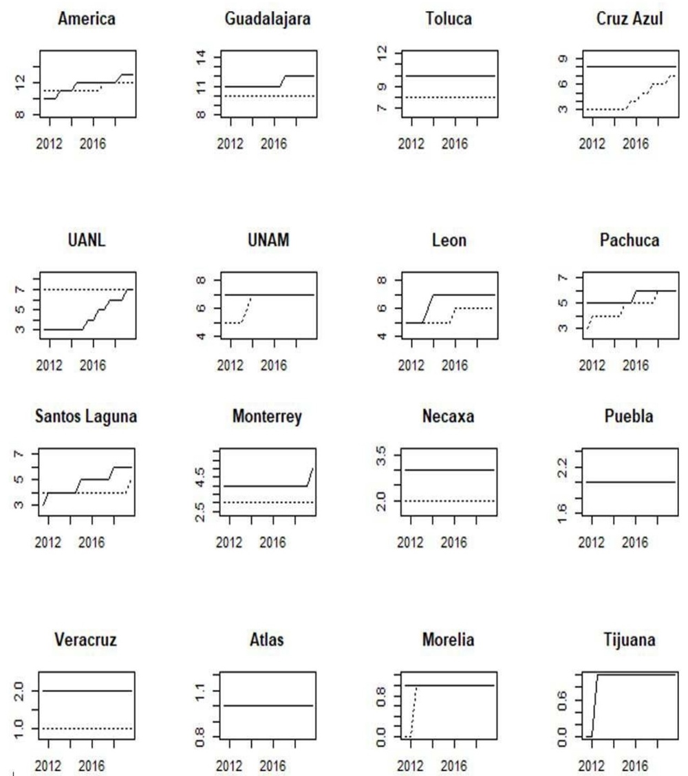
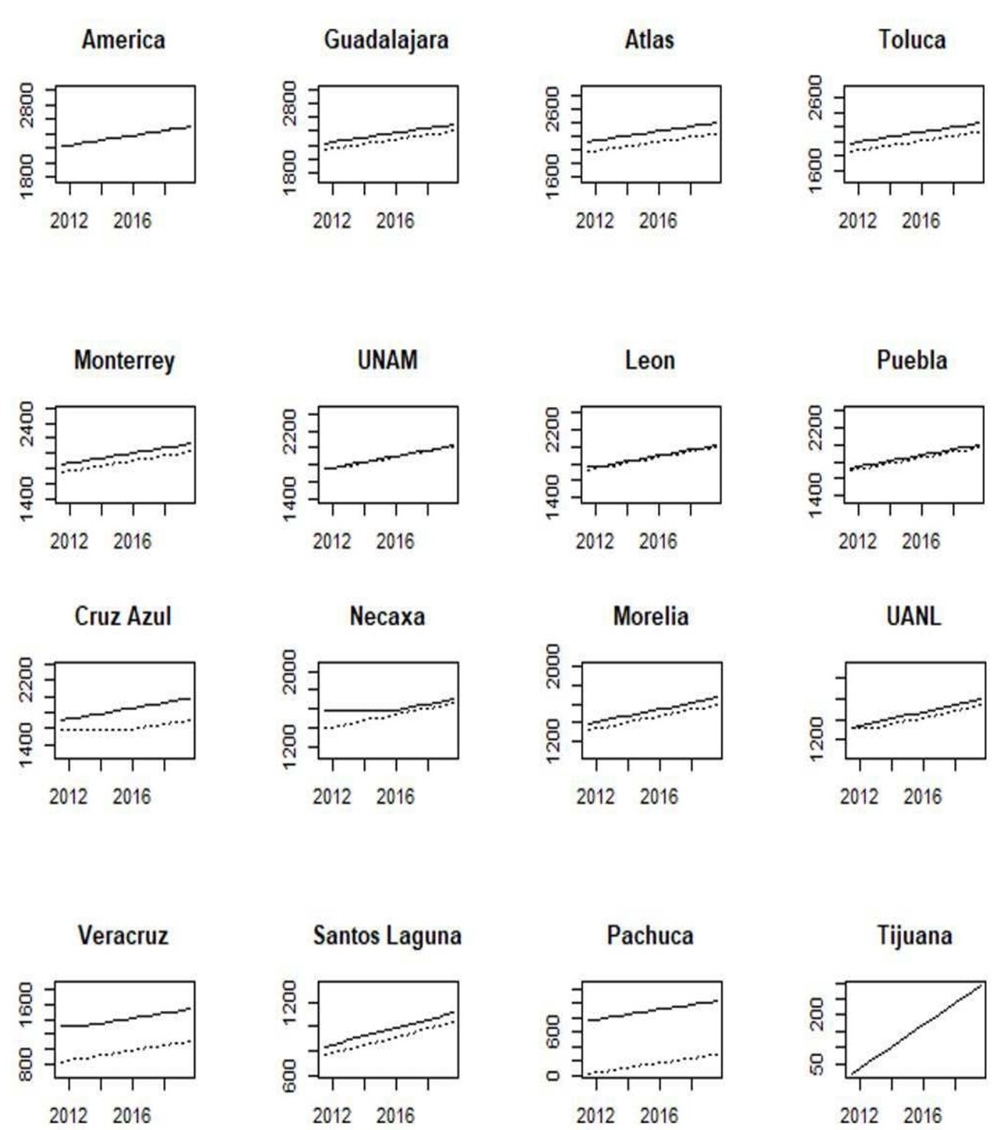
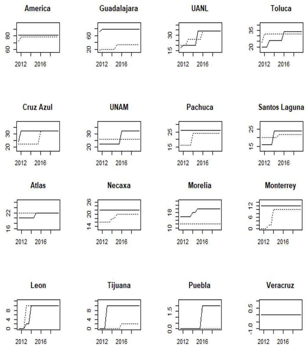
This subsection is based on a set of graphs for the incumbent seasons. These are shown in appendixes: A for domestic tournaments, B for international tournaments, and C for popularity and finance-related variables. We plot each data set according to our ranking as of Apertura 2019 by using solid lines. Additionally, within each plot, we jointly included the adjacent team in the ranking using dotted lines. As mentioned before, the richness of the data used to measure teams’ domestic performance relies on its stock accumulated nature rather than a flow nature; thus, although the period under consideration is from Apertura 2011 to Apertura 2019, they show the cumulative performance since Liga MX inception, back in 1943, allowing thus a long-term appreciation of the football history in Mexico. This way, we avoid structural changes in data that can arise due to changes in the league’s configurations. For instance, before 1970, the league’s configuration was like a pure league competition, where the team that finished at the top of the table was declared the winner; also, since 1996, short tournaments were put in force, which consisted of two tournaments in a year, doubling the number of championships available. Until the 2000s, there existed three groups in the regular season, and the top 2 teams of each group passed to the next phase, disregarding if their performance was poorer than other teams with more points in other stronger groups, which in the end gave room for free-rider teams within weak groups.
We see, in particular, that the metric of Titles (figure A.1) shows very low variability, as only one team wins another title any given season. Nonetheless, this statistic is ultimately representative of overall performance. Note that América has the most wins, followed by Guadalajara, Toluca, and Cruz Azul. It is interesting to note that UANL is the team with more growth during this period. The number of Games Played (figure A.2) accounts for constant participation in the league and is merely affected by relegation. América and Guadalajara are the only teams that have remained in First Division throughout the professional era.
The Points variable is measured as cumulative points divided by cumulative games. It can be considered a measure of teams’ handicap, as it summarizes the number of wins, draws, and losses adjusted by the number of games played throughout history. The most recently promoted team, Tijuana, exhibits the best figures, given its short tournament history. Surprisingly, teams with renowned history are surpassed by more modest teams like Cruz Azul and Santos (figure A.3).
Contrary to GP, the GP-P variable (figure A.4) is related to performance in the knock-out phase. This variable allows us to differentiate between top and low performers: while top teams’ main goal is to compete for championships, more modest teams’ main objective might be merely to qualify for the second phase, while lower teams rarely see their figures moving. América, Cruz Azul, and Toluca are the teams with more participation in the play-offs.
Copa MX is a traditional tournament played since the league’s creation in 1943, despite a lengthy hiatus that lasted from 1997 to 2012. We mean the tournament where First Division teams (Liga MX) meet Second Division teams (Ascenso MX, figure A.5). Its format has also changed over the years. However, the most competitive teams involved in international tournaments are not considered. América, León, and Puebla are the teams with more championships.
Mexican teams’ participation in the international arena is a way to benchmark domestic performance relative to clubs abroad: North America’s CONCACAF Champions League (figure B.1), South America’s CONMEBOL Libertadores, Copa Sudamericana, and Copa Merconorte (figures B.2 and B.3). Thus, despite these variables exhibiting relatively low variability, their inclusion in the analysis is crucial to cast attention on international competitiveness. It is noteworthy that Mexican teams have been banned from participation in CONMEBOL’s tournaments since 2016 due to nonconformities with the competition’s fixtures. Popularity polls across time show that, with slight variations across them, the top 4 remain unchanged: América, Guadalajara, Cruz Azul, and UNAM (figure C.1). As a proxy for market share, popularity is relevant for teams in terms of expected revenue due to merchandise and jersey sells. This variable looks pretty reactive to championships won. For example. América’s popularity clinched right after Clausura 2013, Apertura 2015, and Apertura 2019 championships; similarly, it picked up for UANL after its recent championships in the second part of the 2010s. An interesting characteristic of Liga MX’s fandom is that popularity is not directly translated into stadium attendance (figure C.2), only the northern teams Monterrey and UANL have capitalized on it by constantly selling out their season tickets. Given the high popularity of soccer in Mexico and the current team’s venue capacity, soccer attendance in Mexico is considered mildly low. It might be explained by low per capita income and difficulty accessing stadiums. Teams have room for improvement since higher attendance is usually related to better home advantage. Note that the roster’s market value (figure C.3) reflects not only investment in players’ acquisition but is also adjusted up by players’ revaluation and adjusted down when players are sold to profit from them. Low-tier teams sell to high-tier ones, while the latter usually sell abroad to Europe or the United States leagues. This is the main source of income generation for some teams, like Atlas or Necaxa, that are not usually fighting for championships.
Looking at the different metrics available for Liga MX, we see that no single team unequivocally dominates all the dimensions or categories considered in this work.
3. Explanatory analysis: Are the number of titles related with the rest of sporty and non-sporty variables in Liga MX?
Clearly, the concept of “greatness” is related to the number of sports titles. Liga MX differentiates from European and South American leagues, in that the continental tournament is not the main reference but the local one, given the relative weakness of CONCACAF teams to Liga MX. For example, in the men’s FIFA/Coca-Cola World Ranking, Mexico’s national team occupies eleventh, while the rest of the national teams are not in the top 20 (as of February 2020). Although the performance of national teams does not directly indicate the competitiveness in domestic leagues, it is reasonable to expect that it is correlated with the league’s competitiveness. Nowadays, the CONCACAF Champions League has acquired more relevance because of the classification tournament to the FIFA Club World Cup competition. However, for Mexican fans the focus is on the domestic tournament in relation to the continental championship.
Since the season 1970-1971 in Liga MX, the championship is not awarded to the club that reaches the most points; the champion is rather decided in a play-off phase, named Liguilla. Nowadays, the second phase starts with eight qualifying teams playing two-legged ties with the winner on aggregate-score progressing. An interesting question is: Are teams benefited from this competition system? There is an idea in Mexican media that América is the “Animal de Liguilla” (play-off beast).12 This idea is often based on the fact that América is the winner of most Liguillas. However, it only has one more title than Guadalajara and three more than Toluca. Table 1 compares official championships and the highest-ranked club in the regular season in the professional era for the sample of teams considered in this work to better understand which teams have benefited the most from the competition system of Liga MX.
Table 1 Comparison between official championships and highest-ranked club in regular season from season 1943 to Apertura 2019
| Team | Official | championships | Table leader |
| América | 13 | 15 | |
| Guadalajara | 12 | 12 | |
| Toluca | 10 | 8 | |
| Cruz Azul | 8 | 13 | |
| León | 7 | 7 | |
| UANL | 7 | 5 | |
| UNAM | 7 | 4 | |
| Santos Laguna | 6 | 3 | |
| Pachuca | 6 | 3 | |
| Monterrey | 5 | 4 | |
| Necaxa | 3 | 1 | |
| Puebla | 2 | 2 | |
| Veracruz | 2 | 3 | |
| Morelia | 1 | 2 | |
| Atlas | 1 | 2 | |
| Tijuana | 1 | 2 | |
| Total* | 91 | 86 | |
Notes: Five teams outside the sample would have won the championship by Table Leader criteria. Source: Authors’ elaboration.
The table suggests that América, Cruz Azul, Veracruz, Morelia, and Atlas are not benefited because they have more leaderships under Table Leader criteria than official championships. On the other hand, UNAM, UNAL, Santos Laguna, and Pachuca, seem to be enjoying the most benefit; the last three being emergent teams since the implementation of “short tournaments” in 1996. Note that under the traditional format of Table Leader to declare the champion team, Cruz Azul would occupy the second place in the ranking and Guadalajara the third. In both cases, América would remain first in Liga MX, although it would have more titles under the traditional system. It is interesting to comment that the Spearman correlation between the two columns of table 1 is 0.91. Note that this equilibrium can be interpreted as a long-term phenomenon since although the leadership team in the regular season is not necessarily the champion, it tends to coincide as an overall statistic.
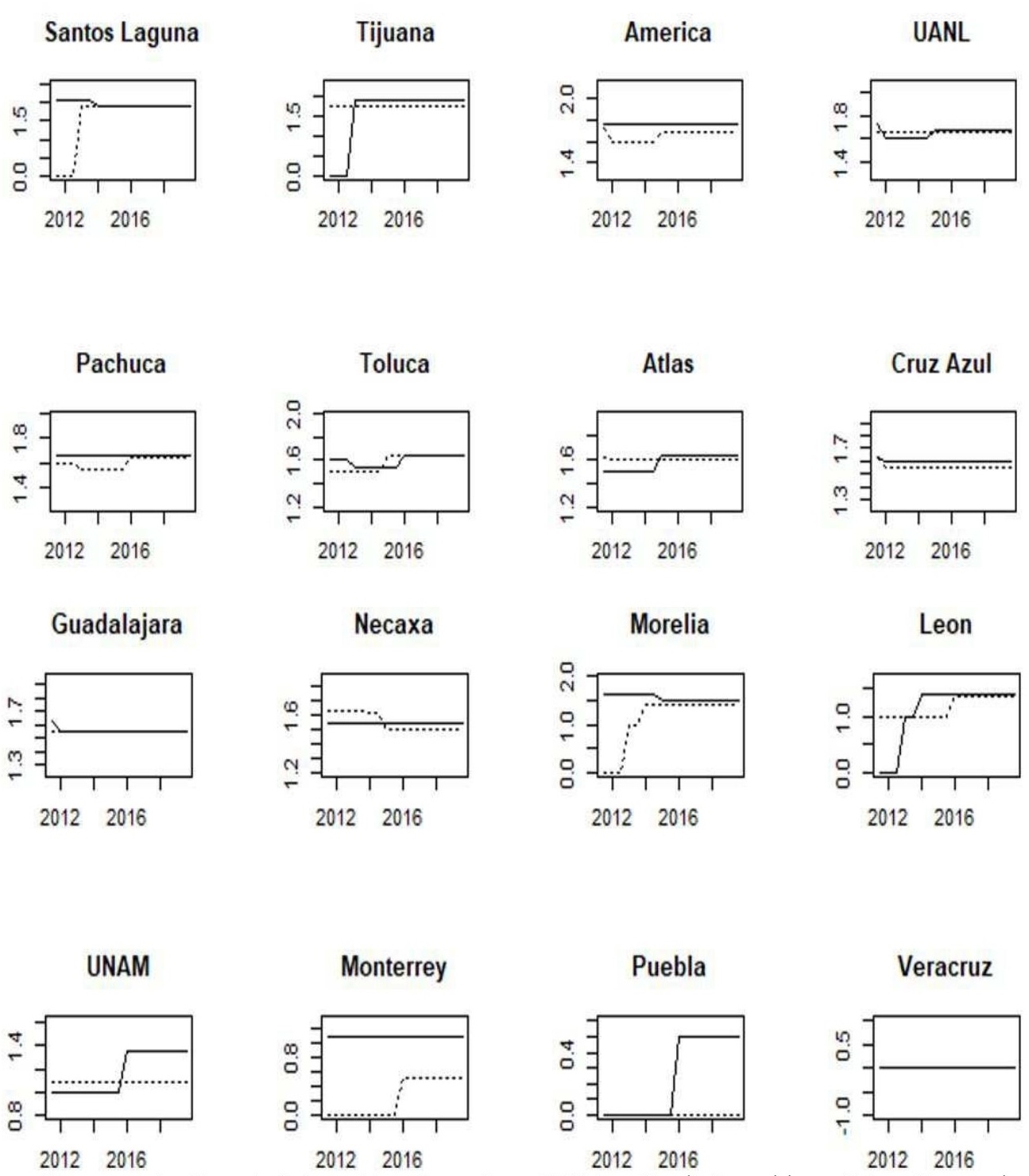
It is interesting to study the relationship between each variable considered in this work with the variable Titles to verify whether all features are positively and significantly related to the championships. Figure 1 shows the results for each pair of linear regressions between Titles and the rest of the variables considering results until Apertura 2019.13
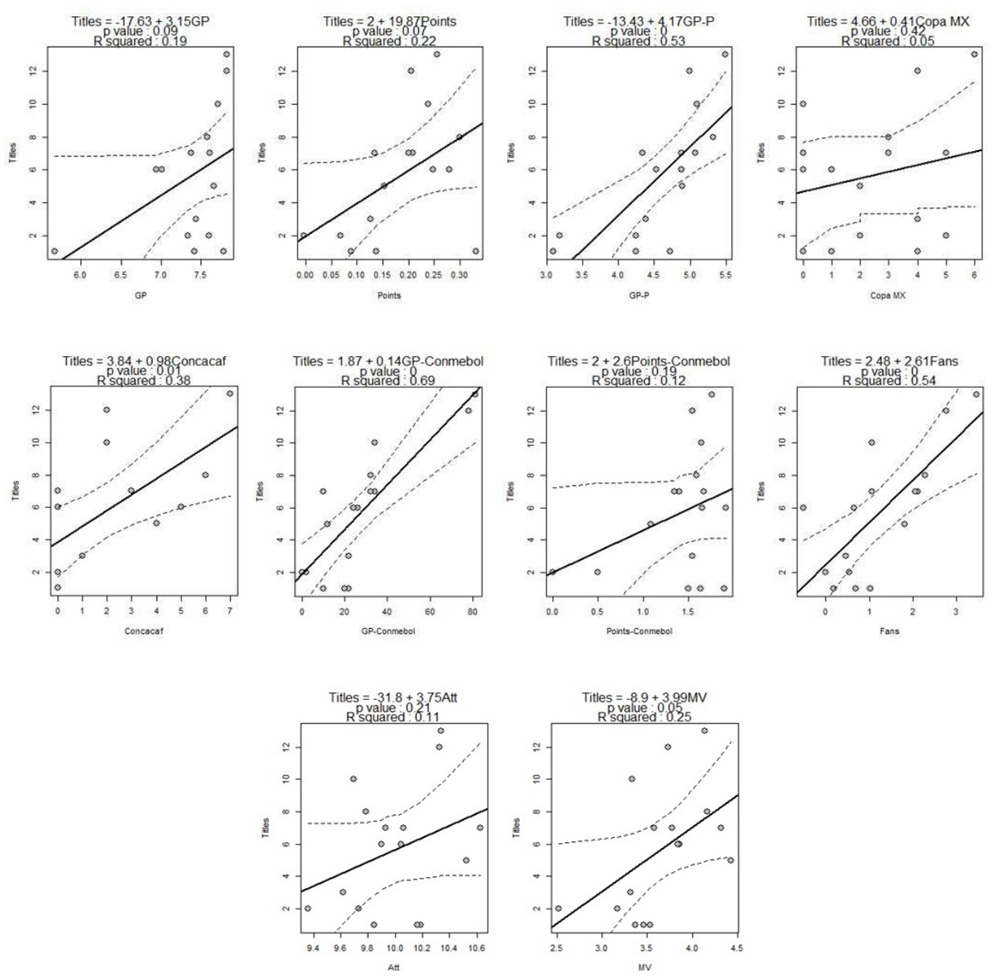
Source: Authors’ elaboration.
Figure 1 Linear regressions between Titles and rest of variables.Apertura 2019
Note that using a 5% of significance GP, GP-P, CONCACAF, GP-CONMEBOL, and Fans are significant. The teams with more titles also have more appearances in CONCACAF and have had more chances to qualify for South American tournaments, and therefore, the number of fans has increased most. Considering a 10% of significance, the number of points in the regular season and the market value of the franchises are also significant. At the same time, Copa MX titles, Points-CONMEBOL, and attendance are not relevant. Under this bivariate point of view, we observe that the number of domestic titles is an important attribute, but not the only one to be considered; as commented before, “greatness” is a latent variable that emerges from the multivariate correlated variables in matrix X.
4. Results: PCA estimation
4.1 Number of components and estimated loadings
First, it is necessary to define the number of factors r in each
tournament. Note that having more than one latent factor complicates the
structural explanation of the principal components because they depend on a
selection of a particular rotation. This issue is not particular to our problem
but is common when using PCA to analyze multivariate data. See, for example,
Bai and Ng (2013) in the context of
large DFM. However, when there is only one principal component, that is, when
The results indicate that the first principal component explains the 42% to 52%
considering all competitions, such that
With this value of

The coefficients are stable in time, although the intervals vary. In all cases, the most important variables are titles, GP-P, GP-CONMEBOL, and the number of fans. On the other hand, the less relevant variable is Copa MX. These results indicate several essential issues, high-lighting the fact that the number of championships, the presence in play-offs and South American competitions, and the number of fans reflect in a better way a combination of sports performance and popularity. Particularly, in Liga MX, a higher presence in play-offs implies more chances of winning, and also, participation in the extinct South American competitions implies the internationalization of the Mexican teams and is related to the attraction of fans. Note that performance in CONCACAF, CONMEBOL, and the MV are also relevant, adding a financial element to the latent variable. Additionally, it is clear that the domestic cup, Copa MX, is not relevant over time. One reason might be the relatively small importance that this competition has for the teams and the fans; as mentioned before, this competition was suspended between 1997 and 2012.
4.2 “Greatness” measure
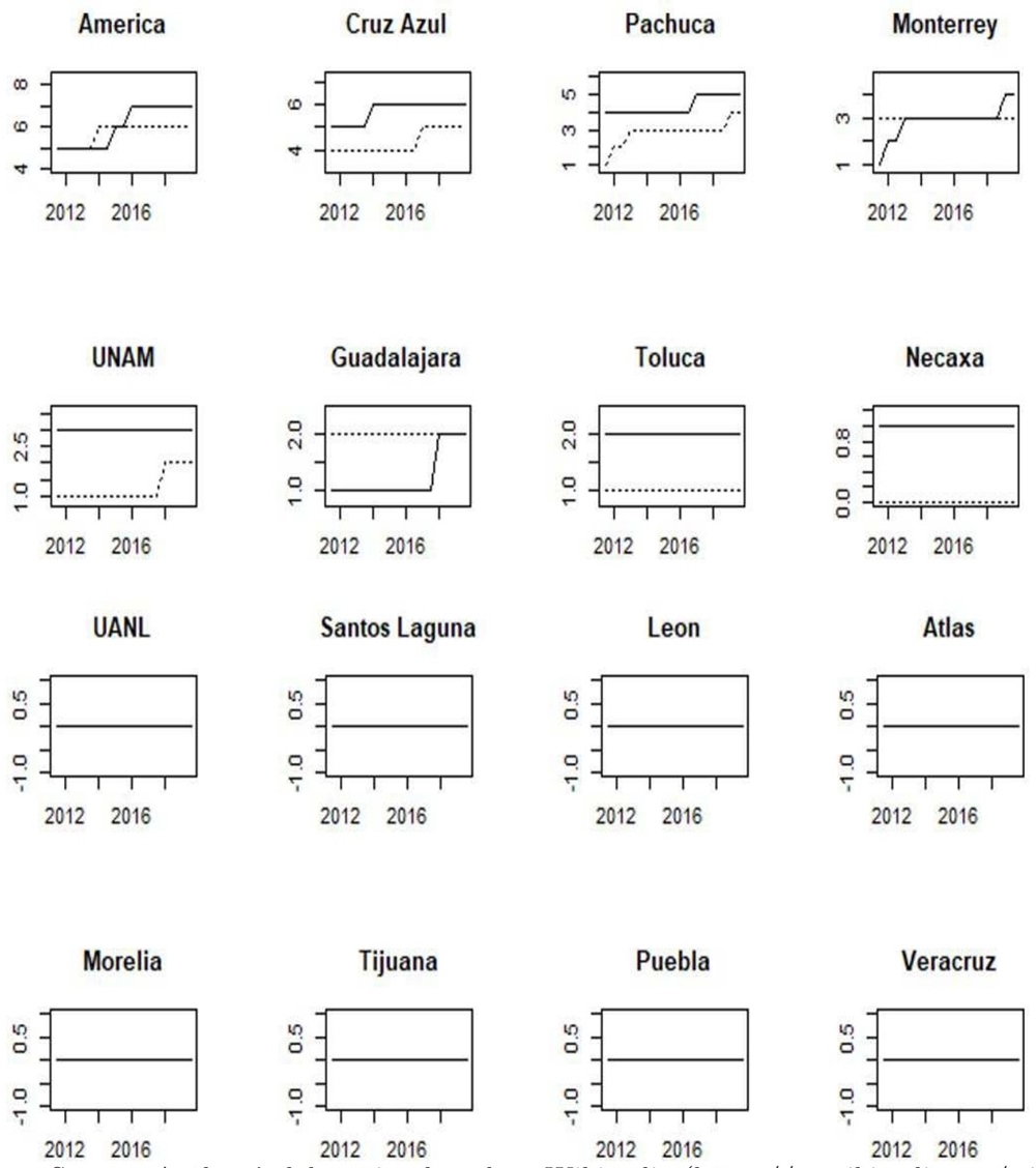
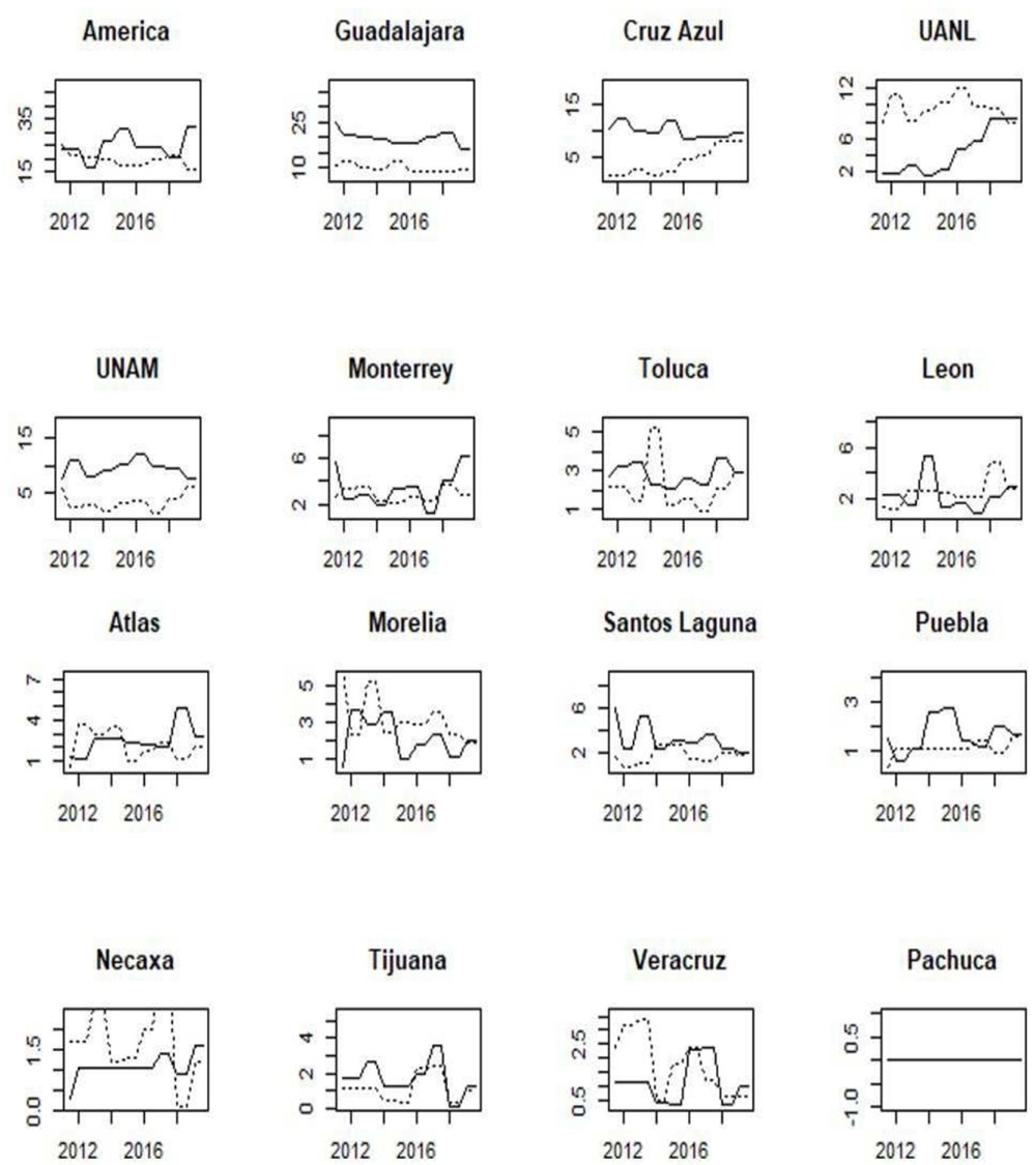
Once each variable’s contributions are analyzed in the latent variable, we extract the factor during time to describe the “greatness” along the competitions. The confidence intervals are also estimated via Bootstrap, similar with the procedure described previously for the factor loadings.14 Figure 3 shows the results.
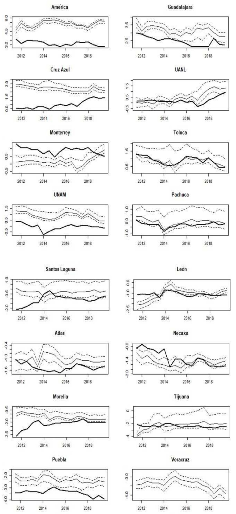
Source: Authors’ elaboration.
Figure 3 “Greatness” measures (solid lines with confidence intervals at 95% in dotted lines) from the top team to the worst team (bold lines) since Apertura 2011 to Apertura 2019
Definitely, the greatest team is América, followed by Guadalajara and Cruz Azul. América is the team with more national and confederation zone championships, games played in First Division (tied with Guadalajara), and games played in play-offs and South America. Additionally, it is the Club with more number of fans. In almost all the dimensions considered, Guadalajara and Cruz Azul are second or third.
The confidence intervals at 95% of the scores of América, Guadalajara, and Cruz Azul do not intersect with the adjacent competitor. We can conclude that, statistically, América has a better performance than Guadalajara, Guadalajara than Cruz Azul, and Cruz Azul than
UANL.
To claim that UANL is “the fourth big team”, we state the following from the results:
Given the pairs of adjacent teams, we can conclude that the intervals of UANL, Monterrey, Toluca, and UNAM intersect in some periods.
UANL and Monterrey have exhibited a positive break since 2017.
Focusing on Apertura 2019, the lower interval of UANL slightly touches the estimated value of Monterrey.
For the same tournament, Monterrey’s lower interval differs from Toluca’s estimated value.
The measures of Toluca and UNAM are statistically equal over time.
UNAM’s measure is statistically different from the values of Pachuca.
Currently, UANL tends to be the “the fourth big team”, followed by Monterrey, while Toluca and UNAM have a similar performance. Before 2017, Toluca and UNAM had a better performance than UANL and Monterrey. Consequently, the measures tend to have changed.
The uncertainty attributed to the estimation does not allows us to conclude on current significant differences between the rest of the teams (without including Veracruz). However, another interesting evolution in the ranking is Tijuana, which in eight years in the professional First Division has evolved from the 16th to the 14th position in the ranking, given its title in Apertura 2012 and for the recent behavior in popularity and financial variables, displacing teams such as Puebla and the recently relegated and extinct team, Veracruz. Pachuca, Santos Laguna, and León are strong competitive teams, but Pachuca and Santos Laguna have been emergent teams since the 2000s and 1990s decades, and Leon was relegated between the 1980s and 2000s. Teams like Atlas, Necaxa, and Morelia lack titles and popularity. Atlas has not won a championship since1950. Necaxa only performed well in the 1990s decade, emigrating from Mexico City to Aguascalientes and was relegated two times during the 2000s. Moreover, Morelia only won one championship in the Invierno 2000 season.
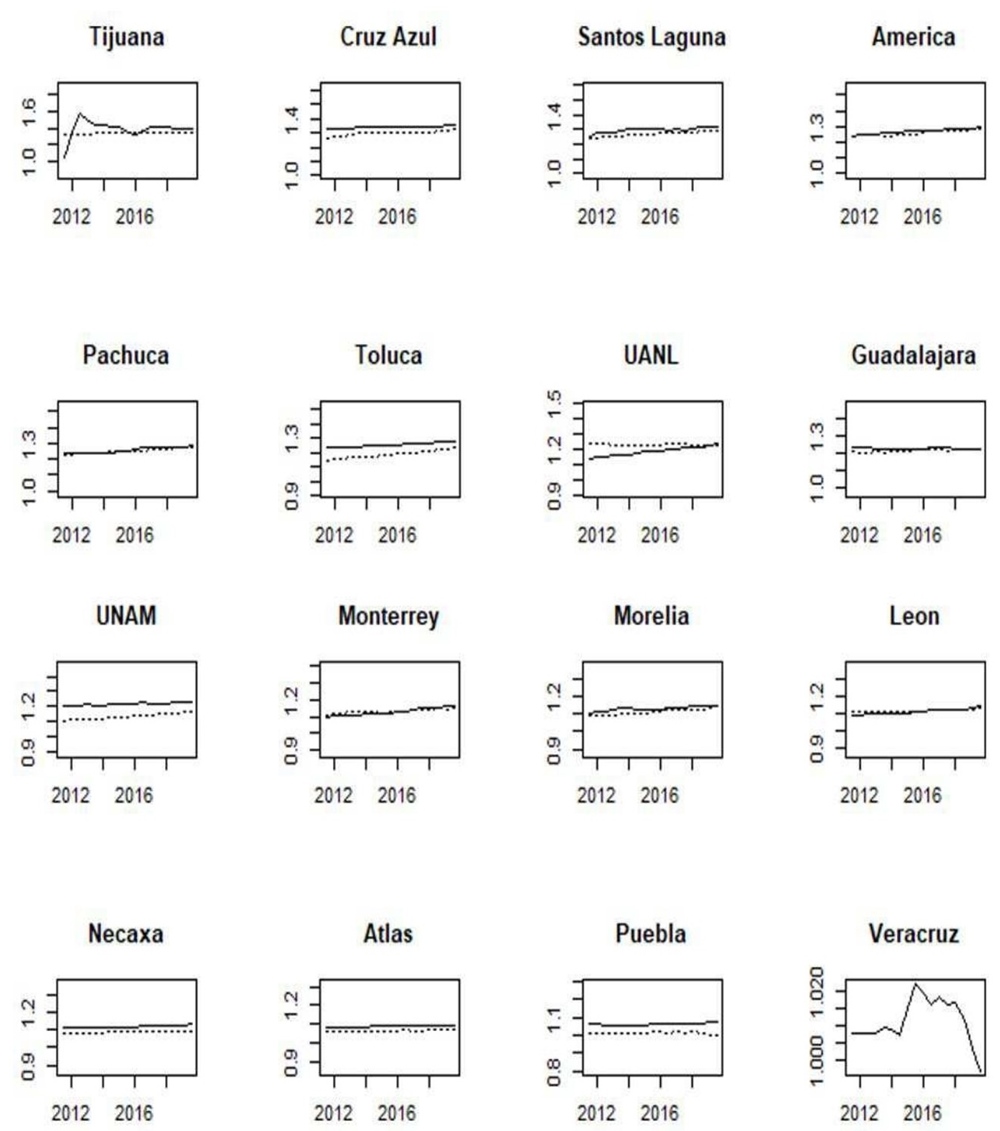
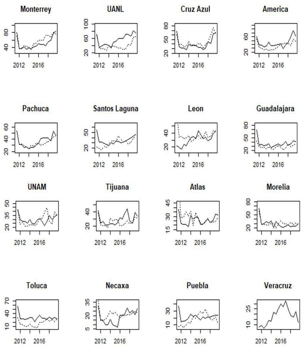
An interesting question arises: What is the role of the non-sporty variables in the ranking? Is it possible to estimate a measure of “greatness” only with sporty variables? To address this, figure 4 presents the factor estimates without popularity and financial variables, along with the full estimations (as in figure 3).

Source: Authors’ elaboration.
Figure 4 “Greatness” measures considering only sporty variables (solid lines).Between parentheses are the correlations with their respective “greatness” measures estimated by using all variables (dotted lines)
From this set of graphs, we acknowledge the importance of popularity and financial variables. The ranking is very different in several cases, not only in levels but also in dynamics. For example, América, Guadalajara, UANL, and Monterrey are the most benefited by the inclusion of the popularity and financial variables, but Cruz Azul, Toluca, Pachuca, and Necaxa are the least ones. Also, the linear correlations between both factors tend to differ in almost all cases. We conclude that our “greatness” measure exploits, in a better way, the dynamics among sporty and non-sporty variables to generate a robust ranking of teams. Our basis for this conclusion is the following: 1) the AIC criterion and ER procedure detect one principal component in several cases; therefore the variables can be summarized in a latent variable, 2) the variables are significant, and 3) the “greatness” measure allows us to determine some statistical differences between the teams.
Our results are amenable to some statistical discussion. For instance, note that the PCA estimates carried out in this work do not assume the dependency on time existing in the database. Consequently, we only model the correlation between variables but assume indepen-dence in time. That is, we assume tournaments to be independent, and this helps us estimate the scores and create time series with these estimations. We implement DFM by using our “greatness” measure to verify the consistency of the estimations over time. Corona et al. (2021) study the stochastic nature of the common factors by using the performance points during short tournaments. Hence, we estimate common factors by asymptotic principal components (PC) and apply Panel Analysis of Nonstationarity in Idiosyncratic and Common components to the estimated common factors and the idiosyncratic errors (Bai and Ng, 2004). More explicitly, after Onatski’s (2010) criterion detected common factors, PANIC tests help us conclude that these factors are non-stationary, whereas the idiosyncratic errors are stationary. This analysis implies that the measures of “greatness” are cointegrated, which implies that applying principal components along the time dimension does not destroy the autocorrelation structure, keeping the common non-stationary dynamic of the set of variables. Furthermore, the common factors estimated by asymptotic PC are robust to some structural changes and sometimes varying coefficients (Stock and Watson, 2011).15
5. Conclusions and further research
The paper represents the first statistical research to answer the question: Who is the greatest team in Liga MX? This question is very attractive in sports media, which answer is usually based on intuition or subjective ideas. It is convenient to note that Liga MX has not been studied enough from an econometric and statistical point. Thus, this paper presents one of the first attempts to measure a ranking of competitiveness by using sporty and non-sporty variables denoted in this work as “greatness”.
Using web-scrapped data, this paper applies PCA for a group of databases of Liga MX historical cumulative results since 1943, updated at every end of season from 2011 to 2019. The analysis of such temporal variability allows us to appreciate the evolution of the greatest team and its relatives over time.
We detect the number of principal components that summarizes this information for all competitions, concluding that with one factor, we can represent the original variability of the dataset at all the time, which facilitates the interpretation of the results. The factor loadings indicate that the most important variables are the games played in play-offs, the domestic titles, the games played in CONMEBOL, and the popularity. Also, the market value of the franchises tends to be relevant. On the other hand, the smallest important variable is the number of titles in Copa MX. Thus, América is the greatest team in Liga MX, followed by Guadalajara and Cruz Azul. A significant result indicates that UANL and Monterrey have overcome teams such as Toluca and UNAM. Note that this exercise shows the evolution of a greatness measure in Liga MX, allowing us to analyze the dynamic the teams along the time for a latent concept. We faced limitations in including financial and popularity measures since they are only available from 2010 and sporty data are available for every season since 1943. However, we consider that “greatness” should involve non-sporty data as well. The trade-off pays in favor of a shorter period but a much richer database that gives an added value relative to similar studies on sport economics.
As further research, we can include other variables in our factor as topics extracted from Google Trends, analyze the prediction capability in statistical models, and also expose the results in sports media TV and sponsors to analyze the relationship between our measure with other financial variables, as broadcasting rights payments and total value of the franchises, and analyze the second and third principal components since some criteria suggested more factors similarly as the dynamic analysis provided by the DFM. Additionally, it interesting to analyze the stochastic nature of the estimated common factors using the “greatness” measures, disentangling the reasons of the possible structural breaks occurred mainly since 2017.