nueva página del texto (beta)
 Inglés (pdf)
 Artículo en XML
 Referencias del artículo
 Enviar artículo por email
 Citado por SciELO
  Similares en
SciELO
Similares en
SciELO 
 Permalink
1. Introduction
In recent decades, income inequality and wealth inequality have increased. This topic has received a great deal of attention in economic literature, both theoretical and empirical.1 This spike in the literature on inequality reached its peak following the publication of Capital in the Twenty-First Century by Piketty (2014), which ignited a heated debate on the validity of the various hypotheses put forward in the book.2
Piketty projects that wealth inequality will increase into the 21st century, his hypothesis being that a larger gap between the return on capital/wealth and the growth rate (hereafter r-g) leads to a rise in wealth inequality.3 The intuition is that the wealth trajectory of the wealthy is determined by r and that of the poor by g. The gap between r and g has been large in the recent past, and Piketty argues that it will remain so.
We use an IV approach and United States (US) data to determine whether a causal relation exists between r-g and wealth inequality. Wealth inequality is measured as the wealth share held by the wealth-iest 1%.4 The US is the only country for which a long-time series of wealth shares and r-g are available. To be precise, we use 84 years of data from 1928 to 2012. Our main data set stems from Saez and Zucman (2016), who use capitalized income data to back out the wealth shares of different percentiles and the percentile-specific returns on wealth and savings rates.
We find a positive and statistically significant relationship between r-g and wealth inequality that is quantitatively relevant. The average increase in r-g of some 4 percentage points from 1928-1976 to 1977-2011 is able to explain between 47 and 52 percent of the recent change in the wealth share of the top 1% (which fell by 0.42 percentage points per year on average between 1928 and 1976 and has increased at an average annual rate of 0.47 percentage points ever since). Therefore, we believe it is essential to understand why the trajectory of r-g changed in recent decades in order to understand the rise in inequality during this period.
We wish to emphasize two caveats that are essential to obtain the correct econometric specification. First, we use the change in wealth inequality rather than its level. The reason is both theoretical and empirical. Theoretically, r−g is related to a change in wealth inequality, not its level. Empirically, wealth shares are nonstationary. The regression of a nonstationary variable on a stationary one may lead to an invalid inference.5 The reason is that one cannot determine any observation as high or low for a nonstationary process as such a process is not mean reverting. Therefore, one cannot establish any meaningful geometric relationship between such a process and a stationary one that is mean reverting and hence whose observations can be described as high or low with respect to their mean. In order to draw a valid inference, we first apply differences to wealth shares. Then, both processes are mean reverting, and a geometric relationship between them can be established. We document that income shares in the US are also nonstationary. This calls for caution regarding the numerous results in the literature on levels of inequality that fail to account for the trending behavior of inequality.
Second, an IV specification is necessary due to endogeneity concerns, particularly reverse causality. There exists a large amount of literature that attempts to determine whether inequality fosters or impedes growth.6 These studies suggest an issue of reverse-causality, though the literature is inconclusive as to the direction of the bias. We use an instrumental variable approach to control for the endogeneity problem. The instrument used is the defense news series developed by Ramey (2011). This series uses a narrative method to measure the expected discounted value of government spending changes due to foreign political events. It was originally created as an instrument to estimate the government spending multiplier.7
We develop Piketty’s hypothesis theoretically to determine the correct empirical specification. First, there is a relation between the change in wealth inequality and r-g. Second, the savings rate should be included in the regression. Moreover, we find that inequality has a cyclical component which could bias the inference; we employ 3-year averages to account for cyclicality.
In both the ordinary least squares (OLS) and IV specifications, we find a positive and significant impact of the percentile-specific rg on the change in the percentile wealth share (for the top 0.1%, 1%, and 5%). An extensive set of robustness checks confirms these results. The savings and marginal tax rates are also significant and display the expected signs. These findings are remarkable given the low number of observations (in most specifications, we are left with 28 observations).
Finally, we run separate regressions for r-g and g to observe whether the results are only driven by an effect of g on inequality. The R2 of r-g is much higher than that of g alone. This implies that the results are not merely due to the effect of growth on wealth inequality but also to the important role played by the difference r−g. This work relates to the influential book by Piketty (2014) and related articles by him and his coauthors, who gathered and estimated historical data on the evolution of wealth and income.8 Importantly, Piketty (2015a) clarifies certain misreading of Piketty (2014) and emphasizes the fact that he does not hold the view that r-g is the only force that drives income inequality. Piketty and Zucman (2015) provide a more detailed analysis of the evolution of wealth inequality and the theory that relates r-g and wealth inequality. Saez and Zucman (2016) use the capitalization technique first developed by King (1927) and Stewart (1939) to estimate the distribution of US wealth since 1913. We rely mainly on their data set in our estimations. Jones (2015) highlights some of the key empirical facts of the research by Piketty and his coauthors, and comments on how these relate to macroeconomics and economic theory in general.
Numerous articles have tackled specific aspects of Capital in the Twenty-First Century. While Krugman (2014) and Solow (2017) provide mostly positive reviews, many scholars challenge one or several of the book’s theories. As Krusell and Smith Jr (2015) note, Piketty advances two central hypotheses in his book. One considers the evolution of the capital-income ratio, and the other relates r-g to inequality. Although somewhat related, these theories have very distinct elements. Krusell and Smith Jr (2015) question the validity of the first hypothesis, whereas the present paper addresses the second.
Rognlie (2014) argues that empirically realistic diminishing returns to capital accumulation imply that the gap will decrease over time and claims that the observed non-decreasing returns to wealth accumulation in recent years are due primarily to the fact that housing wealth increased. Mankiw (2015: 43) argues that: “The first thing to say about Piketty’s logic is that it will seem strange to any economist trained in the neoclassical theory of economic growth. The condition r>g should be familiar. In the textbook Solow growth model, it arrives naturally as a steady-state condition as long as the economy does not save so much as to push the capital stock beyond the Golden Rule level [...]”. Moreover, Mankiw (2015) claims that while Piketty’s theory that a large r-g can increase inequality is true in principle, the differences in r and g required to cause an increase in wealth inequality greatly surpass those empirically observable (he suggests instead that r−g > 7% is necessary). In contrast, we analyze empirically whether the levels of r-g observed in the 20th century can explain changes in wealth inequality.
Ray (2015) argues that a large r-g does not necessarily lead to an increase in wealth inequality. Instead, he asserts that all that mat-ters is the fraction of r that capitalists save, and the relevant equation would have to be 𝑠𝑟>𝑔, where s is the savings rate. He further argues that this only leads to increasing wealth inequality if capitalists represent the richest agents in the economy. Moreover, Milanovic (2016) argues that greater capital share and increased interpersonal inequality are not as simple and unambiguous as it seems and considers that, even when the positive relationship between the two exists, the strength of that relationship varies. While these objections are certainly true, it is indisputable that capitalists are proportionally overrepresented in the top wealth quintiles, as Piketty empirically shows. Furthermore, an increase in r-g tends to raise 𝑠𝑟−𝑔. However, we control for the quintile-specific savings rate in our analysis, as we agree with Ray (2015) on this issue.
One extensive critique of Piketty’s theory is that of Acemoglu and Robinson (2015), who consider institutions to be the predominant factor in explaining inequality. It is difficult to always distin-guish between these two mechanisms, as institutions play a significant role in the evolution of r-g. While an interesting topic of study, the role institutions play in the trajectory of r-g is beyond the scope of this paper. Acemoglu and Robinson (2015) argue that r−g is not related to inequality, as they find no positive relation between r-g and top income inequality. Their results beg three comments. First, Piketty argues that it is wealth inequality that is governed by r-g. Income inequality and wealth inequality are only closely related if the persistence in the income process is sufficiently strong. Second, the relevance of the proxies that Acemoglu and Robinson use for r, GDP growth rate, government bond yields,9 and marginal product of capital could be questioned. The later proxy, marginal product of capital, seems to be the best, and when they use it, they find some evidence of a positive relation between r−g and inequality. Third, we find wealth and income shares to be non-stationary, which may imply that using inequality levels leads to an invalid inference.
The work most closely related to ours is that of Fuest et al. (2015), who aim to test the relation between r−g and wealth inequality and also find a positive relationship.10 Instead of time series data, they use panel data, the advantage of this being that they have more observations, though at the cost of not having a common measure for the return to capital r. However, there are a few deficiencies regarding that article. In place of r, they use a financial development indicator as a proxy that is more of an institutional variable, and it is unclear whether financial development induces r to increase or decrease.11 Furthermore, they regress the wealth share on g and their financial development indicator separately. Finally, in contrast to our work, they do not employ an instrumental variable approach and, therefore, cannot address the endogeneity issue.
The remainder of the paper is structured as follows. In section 2 we develop Piketty’s hypothesis analytically to provide a theoretical underpinning for our empirical specification. In section 3, we discuss the data sets employed and the trending behavior of the central variables. Section 4 contains the core results and a battery of robustness checks. Section 5 concludes.
2. Theoretical considerations
Piketty and his coauthors claim that the evolution of wealth inequality depends greatly on the evolution of r−g. The intuition is that r determines the earnings of the wealthy capitalist class and, thus, the growth rate of their wealth. In contrast, g determines the evolution of the wages and wealth of the average citizen who possesses almost no savings. We use a simple theoretical model to clarify the argument and our empirical specification.
Let us suppose there are two types of representative agents -workers and capitalists- at
fractions ε and
Aggregate wealth, WT , can be written as:
The wealth share of capitalists at any point in time is defined as:
The change in time of this ratio is determined by:
that where X denotes the change of the variables X in time. Note
and similarly,
where g denotes the growth rate of labor income and is assumed to be equal to GDP growth (which holds in standard growth theory). This implies that:
Hence, the necessary condition for wealth inequality to increase is:
This inequality reveals two things: First, there is a relation be-tween r-g and the change
in wealth inequality, not the level of wealth inequality. Second, the savings rate alters
the relation between rg and wealth inequality. Therefore, if correlated with
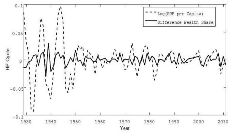
We do not aim to estimate this model structurally, as the model is far too simplistic. Many other factors influence the evolution of inequality, such as government policy, unemployment rates, trade, and so on. Importantly, the change in wealth share displays cyclical properties. We document this in the appendix (A.1). This leads to two concerns. First, the cyclicality augments the variance and thus may lead to erroneous inference. Second, any correlation found between the two variables can be due to a lurking variable driving the cycles of both. We take 3-year averages to account for the cyclicality.14
3. Data
We employ the unique US dataset by Saez and Zucman (2016), who provide yearly wealth shares for different percentiles over a span of almost 100 years obtained using the capitalization technique.15 The dataset also includes national growth rates, and both percentile-specific savings rates and returns to capital. In our central specification, we focus on the top 1% of wealth holders.16 One drawback is that they only provide total real net returns on wealth from 1961 on-wards. Therefore, we construct an approximate time series using the tax rate on capital provided by Piketty and Zucman (2014).17 “Capitalists” (top 1% top rung) may accumulate more claims on productive capital both because the rate of return is higher -which boosts the re-sources available to save from and because their savings rate is higher. However, we emphasize that we do indeed use the percentile-specific savings rate. Saez and Zucman (2016) provide a unique US dataset that contains the percentile-specific savings rates required in our estimation. This is important to avoid the possible misunderstanding related to the fact that a regression of the change in wealth share on r-g and the aggregate savings rate would not warrant causality. To be sure, also the marginal tax rates and the returns on interest are percentile specific.18
We combine this dataset with additional data sources. As a control variable, we include the marginal income tax rate for the top wealth percentiles by combining the average income per wealth percentile provided by Saez and Zucman (2016) and a time series of the federal individual income tax rates history from the US.19 The marginal income tax rate serves as a proxy for government policies regarding redistribution.
We further incorporate the defense news series developed by Ramey (2011) as an instrumental variable in our analysis. When we test for the exclusion restriction, we include as alternative explanatory variables the unemployment rate, the share of government expenditure directed towards national defense purposes, and the ratio of democrats to republicans in parliament.20
An important issue is whether the variables are stationary or not. Only a balanced regression that uses processes with the same trending behavior makes it possible to draw valid inferences. The reason is that -in contrast to a stationary variable- one cannot determine a single observation of a nonstationary process as high or low, as such a process is not mean reverting. Thus, any inference drawn can be invalid when a nonstationary variable is regressed on a stationary variable (Stewart, 1939).21
There is consistent evidence of stationarity for all the variables save for wealth shares and marginal tax rates. For tax rates, the evidence is mixed, whereas for wealth shares, the tests provide evidence in favor of the unit-root hypothesis. The results are summarized in table 8 in the appendix and justify the proposal to first-difference the wealth shares.
Theoretically, we find a relationship between the change in wealth shares and r-g. There is also considerable empirical evidence that wealth shares in the US behave as a nonstationary process, whilst the other variables of interest (growth rate, return to capital, savings rate, and tax rate) are stationary. We apply first differences to the wealth shares in order to be able to draw a valid inference, since the change in wealth shares is a stationary process. The results are summarized in table 8 in the appendix and justify the proposal to first-difference the wealth shares. We extend this result, test US income shares for stationarity, and again fail to reject the unit root hypothesis for income shares. This casts doubt on an array of studies on income inequality that use the level of inequality as the dependent variable.
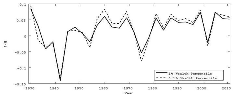
The central time series are depicted in figures 1 and 2. Simple 3-year averages are constructed as the average values of the peri-ods 1928-1930, 1931-1933, 1934-1936,..., 2006-2008, 2009-2011. As a robustness check, we also use moving averages (average values of 1928-1930, 1929-1931, 1930-1932,, 2008-2010, 2009-2011) as well as Hodrick Prescott filters of the variables of interest. Figure 1 depicts the 3-year averages of the wealth share of the top 0.1% and 1%, which display a downward trend until the late 70s and an upward trend thereafter. More specifically, the wealth share of the top 1% dropped 0.416 percentage points on average each year between 1928 and 1978 and increased 0.473 percentage points per year from then on (the last observation dates from 2011). Figure 2 displays the respective 3-year averages of the percentile-specific r-g. This variable displays a lot of variation. On average, r-g rose over time. Prior to 1978, the average r-g was 0.5 percentage points for the top 1% before rising to 4.4 percentage points, where it has remained (on average) ever since. The respective increase for the top 0.1% (10%) is from 0.6 to 5.0 (0.5 to 4.0) percentage points. This is summarized in table 1.

Source: Authors’ elaboration with data of Saez and Zucman (2016).
Figure 1 The wealth shares for different wealth percentiles
Source: Authors’ elaboration with data of Saez and Zucman (2016).
Figure 2 The r-g for different wealth percentiles
Table 1 Average r-g for different percentiles
| 1928 - 1978 | 1979 - 2011 | |
| 0.1% - Percentile | 0.006 | 0.050 |
| 1% - Percentile | 0.005 | 0.044 |
| 10% - Percentile | 0.005 | 0.040 |
Source: Authors’ elaboration with data of Saez and Zucman (2016).
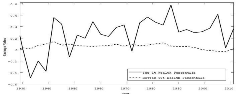
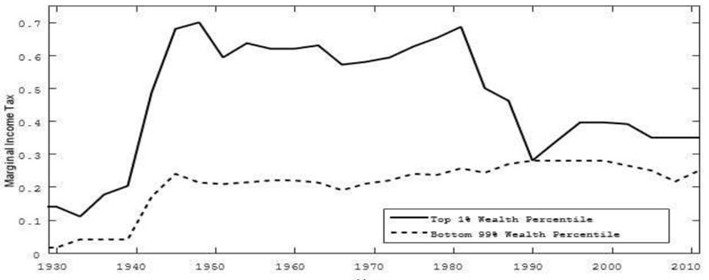
Figures 3 and 4 show the 3-year averages of the savings and marginal income tax rate for the top 1% and bottom 99% of wealth holders. Both rates are nonconstant and differ significantly between the different wealth percentiles. We have shown theoretically that a non-constant savings rate influences wealth inequality and therefore has to be included in the empirical regressions. Similarly, a nonconstant marginal income tax rate has to be included.22 The marginal income tax rate may measure a government’s position towards redistribution.
Source: Authors’ elaboration with data of Saez and Zucman (2016).
Figure 3 The savings rates for different wealth percentiles
Source: Authors’ elaboration with data of Saez and Zucman (2016).
Figure 4 The marginal income tax rate for different wealth percentiles
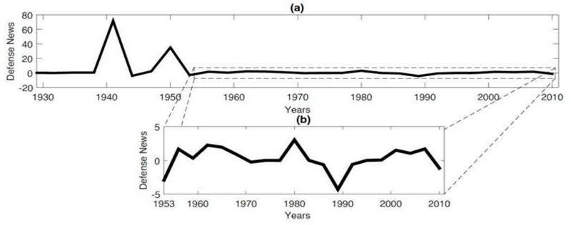
Figure 5 displays the time series of our instrument Defense News. As mentioned, the series constructed by Ramey (2011) is a narrative of the expected discounted value of government spending changes due to foreign political events. The series is constructed by reading periodicals to gauge the public’s expectations. It shows a great deal of variation dominated by two major war events, the Second World War and the Korean War. Panel (a) of figure 5 depicts the entire time horizon, whereas panel (b) focuses on the period after the Korean War to show that there is also substantial variation in those years.
4. Regression results
Before we document the results, let us focus on endogeneity concerns, particularly reverse causality concerns. The economic literature on the effect of inequality on growth is vast yet inconclusive.23 Furthermore, wealth inequality can affect the rate of return r, as it influences supply and demand in the capital market. Hence, endogeneity concerns exist and may be addressed by an instrumental variable approach. Importantly, we cannot attach a priori a sign to the endogeneity bias as it is unclear whether greater inequality leads to a higher or lower r-g. Therefore, estimates from OLS regressions can be upward or downward-biased.
Our chosen instrument is the dataset on defense news provided by Ramey (2011). This dataset has been used as an exogenous instrument to identify the effects of government spending on growth. Defense news causes the government budget to increase, which serves as a stimulus for the entire economy. It is relevant, as shown by Ramey (2011) and our first-stage results. In our central specifications, we include three lags of our instrument as this specification delivers the highest adjusted R2 and F-values. We show the regression results of the first stage in the appendix in table 9.24 This implies that there exists a relationship between defense news and r-g. However, there may be other channels that are affected by defense news and influence wealth inequality. For example, defense news may well affect military spending or unemployment rates and may influence inequality. In the robustness section, we exert several robustness checks indicating that the exclusion restriction is met.
Our two central regressions are:
and
In the second specification, we include the savings and marginal income tax rates. We have
shown that they should be included in a regression as they are non-constant over time and
influence the relation between
Table 2 presents our core regression results: the
regression of the change in wealth percentile on the percentile-specific difference of
return on capital and growth rate. In column 1,
Table 2 Results for 1%-percentile wealth share regressions
| Dependent variable: Change in wealth share | 1 (OLS) | 2 (OLS) | 3 (OLS) | 4 (IV) | 5 (IV) | 6 (IV) |
| r-g | 0.3695*** | 0.3406*** | 0.2732*** | 0.3324*** | 0.3671*** | 0.3523*** |
| (0.0446) | (0.0483) | (0.061) | (0.03) | (0.0391) | (0.034) | |
| Savings rate 1% | 0.0364*** | 0.0366*** | 0.0360*** | 0.0351*** | ||
| (0.0129) | (0.0085) | (0.0131) | (0.0098) | |||
| Marginal tax rate 1% | -0.0482*** | -0.0266* | -0.0470*** | -0.0270* | ||
| (0.0134) | (0.0141) | (0.0138) | (0.0145) | |||
| Crash 1929 | 0.1260*** | 0.1087*** | ||||
| (0.0211) | (0.0175) | |||||
| WW II USA | -0.0048 | -0.0001 | ||||
| (0.0054) | (0.0033) | |||||
| Crisis 2008 | 0.0749*** | 0.0655*** | ||||
| (0.0117) | (0.0099) | |||||
| T | 28 | 28 | 28 | 28 | 28 | 28 |
| R2 | 0.4945 | 0.6553 | 0.7745 | 0.4945 | 0.6544 | 0.7633 |
| Adj. R2 | 0.475 | 0.6122 | 0.71 | 0.475 | 0.6112 | 0.6957 |
| F-Value | 68.61 | 17.85 | 2857.38 | 122.91 | 42.12 | 7665.18 |
| F-Value (1st Stage) | 444.8 | 112.84 | 186.59 | |||
| Hausman-test | χ2 (1)= | χ2 (1)= | χ2 (1)= | |||
| 0.2564 | 0.2439 | 3.1459 | ||||
| p-value= | p-value= | p-value= | ||||
| 0.6126 | 0.6214 | 0.0761 | ||||
| Sargan-test | LM= | LM= | LM= | |||
| 4.3335 | 1.5513 | 2.7296 | ||||
| p-value= | p-value= | p-value= | ||||
| 0.2276 | 0.6705 | 0.4352 |
Notes: Constant excluded, robust standard errors. Standard errors in parentheses. *p<0.1, **p<0.05, ***p<0.01. Source: Authors’ elaboration.
In all regressions, the R2, the adjusted R2, and the F-values are high, which indicates that the model is able to capture a large part of the variation in the change in wealth shares. As for our IV specifications, we fail to reject the null hypothesis of the Hausman test of endogeneity. This is not surprising, as we did argue that the endogeneity bias can go in either direction. In consequence, the different endogenous effects may cancel each other out. Therefore, the failure to reject the Hausman test does not imply that endogeneity is not a concern.
The estimates on r−g are statistically significant and possess high economic relevance.
Multiplying the stated long-term increase in r-g of 3.9 by the yearly β of 0.1073 to 0.1182
yields a projected change in wealth inequality of 0.419 to 0.461 percentage points. This is
between 47 and 52 percent of the observed swing in wealth inequality. Hence, r−g can explain
a large part of the evolution of US wealth inequality in the last decades. Figure 6 provides a scatterplot of the observed and
predicted values. The x-axis depicts the 3-year averages of the 1%-percentile


To determine the driving force behind the results, we want to see the predictive power of the growth rate alone, without the return on capital. Therefore, we run the IV regressions separately using either r−g o𝑟 g alone and compare the explanatory power of both.26 The results of this rat race are shown in table 3. While the growth rate alone is significant, a comparison of the R2 clearly shows that it cannot explain anything close to the variation that r-g is able to explain. This provides convincing evidence that the channel r−g plays a significant role in the process of wealth inequality.
Table 3 Results for 1%-percentile wealth share regressions
| Dependent variable: Change in wealth share | 1 (IV) | 2 (IV) | 3 (IV) | 4 (IV) |
| r-g | 0.3324*** | 0.3671*** | ||
| (0.03) | (0.0391) | |||
| g | - 0.2898** | -0.4582*** | ||
| (0.1349) | (0.1131) | |||
| Savings rate 1% | 0.0359*** | 0.0696*** | ||
| (0.0131) | (0.0229) | |||
| Marginal tax rate 1% | -0.0470*** | -0.0699*** | ||
| (0.01389) | (0.0199) | |||
| T | 28 | 28 | 28 | 28 |
| R2 | 0.4945 | 0.0287 | 0.6544 | 0.2972 |
| Adj. R2 | 0.475 | -0.0087 | 0.6112 | 0.2093 |
| F-value | 122.91 | 4.62 | 42.12 | 9.01 |
| F-Value (1st Stage) | 444.8 | 194.52 | 112.84 | 155.45 |
| Hausman-test | χ2 (1)= | χ2 (1)= | χ2 (1)= | χ2 (1)= |
| 0.2564 | 2.6733 | 0.2439 | 5.8035 | |
| p-value = | p-value = | p-value = | p-value = | |
| 0.6126 | 0.1020 | 0.6214 | 0.0160 | |
| Sargan-test | LM = | LM = | LM = | LM = |
| 4.3335 | 4.1844 | 1.5513 | 2.2056 | |
| p-value = | p-value = | p-value = | p-value = | |
| 0.2276 | 0.2422 | 0.6705 | 0.5308 |
Notes: Constant excluded, robust standard errors. Standard errors in parentheses. *p<0.1, **p<0.05, ***p<0.01. Source: Authors’ elaboration.
4.1 Robustness checks
First, we redo the regression exercise for the top 0.1% instead of the top 1%. Accordingly, we use this wealth percentile’s savings rate and marginal income tax. The results are depicted in table 10 and confirm those found above. In the OLS and IV specifications, r-g is positive and highly significant, the savings rate also has a positive impact, and the marginal tax rate has a negative one. The channel r-g is able to explain between 38 and 48 percent of the recent increase in wealth inequality (redoing the analogous calculation above), a slightly lower share.
Table 11 depicts the regression exercise using the top 5% wealth share. Unfortunately, there is no data for the 5% specific r-g available. Therefore, we use the top 10% specific r-g.27 Again, r-g is positive and highly significant in all specifications. However, both the savings and the marginal tax rates are insignificant in these specifications. This comes as no surprise as both the savings and the marginal tax rates are closer to the mean for those agents. Again, the increase in r−g in recent decades is able to explain between 38 and 42 percent of the increase in wealth that experienced the top 5% wealth percentile.
Our results are not sensitive to including additional lags of the instrumental variable, defense news. In table 12, we include one and three lags of the instrument and show that the results are very similar. The choice of the lags we include is motivated by the F-statistics in the first stage (see table 12). Actually, the coefficients of the variables of interest do almost not change at all. These specifications also allow us to perform the Sargan test of endogeneity. The null hypothesis that the coefficient of the IV specification is equivalent to that of the OLS specification cannot be rejected. In various studies, lags of the independent variables are used instead of instruments to control for endogeneity. Although we clearly prefer the IV approach (as expectations on the evolution of wealth inequality may have an impact on contemporaneous growth and capital market demand and supply), we provide the results for those regressions in columns 5 and 6 of table 12. Again, 𝑟−𝑔 remains significant. The savings rate shows up significantly, whereas the marginal income tax rate does not.
In table 13, we use alternative conceptualizations for 𝑟−𝑔 In particular, total real gross return on wealth and real net capital gains-for which long-time series are provided by Saez and Zucman (2016)-show similar significance and magnitude.
In columns 1 and 2 of table 14, we show that excluding either the savings rate or the marginal tax rate does not substantially change the coefficient of 𝑟−𝑔. In columns 3 to 5, we use the relative savings rate and relative tax rate. More specifically, the savings rate of the top 1% is replaced by the difference in savings rate between the top 1 percent and bottom 99 percent, as differences in savings rates may have more explanatory power. Similarly, we replace the marginal tax rate with the difference between the top 1% and bottom 99% marginal tax rate. Including one or both of the relative rates does not change the significance or magnitude of r-g. Both the relative savings rate and the relative marginal tax rates are of similar magnitude as the absolute values.
We also use different concepts to control for cyclicality. Using either 3-year moving averages or a Hodrick-Prescott filter rather than 3-year averages provides qualitatively similar results (see table 15).28 A clear advantage of these procedures is that we have more observations. The value of β is in a similar range (recall that in order to make the comparison, the ßs in table 15 need to be multiplied by 3 as we used 3-year averages in our main specification). The marginal tax rate loses significance in one HP specification. We have the exogeneity assumption using the Sargan test in 3 specifications. This comes as no surprise, given the large number of instruments.
In columns 1 and 2 of table 16, we show that allowing for a time trend does not change the significance or magnitude of r−g. In columns 3 and 4, we construct sr−g as our theoretical considerations predicted. While we know that the theoretical model was far too simplistic, the fact that sr−g results significant supports Piketty’s r-g hypothesis.
We also address the issue of whether the instrument satisfies the exclusion restriction. The exclusion restriction can never be tested empirically. However, we included a few potential alternative mechanisms as to how defense news influences wealth inequality. Namely, we test whether the inclusion of the unemployment rate, the military spending, and the ratio between Democrats and Republicans change the coefficient of r−g. Conceivably, defense news changes unemployment due to more people entering the military, which may lead to a change in wealth inequality. Similarly, an increase in military spending may affect other social government expenditures which may affect inequality. At last, defense news may cause support among political parties to shift, which may have an influence on inequality. The results are depicted in table 17. The inclusion of any of those variables or all three jointly does not affect the significance nor magnitude of the beta coefficient of r−g. This provides empirical support that the exclusion restriction is met, and wealth inequality is affected by defense news exclusively via r−g.
Finally, we replace the dependent variable, 1%-percentile wealth share, with the Gini index, as the later variable could be considered a better gauge of inequality. Using the Gini coefficient is therefore a valuable exercise.29 The main finding, this is, evidence of a positive relationship between inequality and r−g, is sustained with the Gini index as the dependent variable. One problem with the Gini index in that respect is that there is not a clear choice as to which percentile to use for the savings and marginal tax rates. Therefore, we opted for the top 1% savings rate as our main result. All the robustness checks and a detailed discussion are relegated to the appendix.
5. Concluding remarks
We investigate empirically whether r−g causes an increase in wealth inequality. Using almost a century of US wealth data, together with percentile-specific returns to capital, we find that r−g plays a significant role in explaining the evolution of wealth inequality over the last century. The increase in r−g in recent decades can explain over 50% of the increase in wealth inequality.
However, this does not imply that a future rise in wealth inequality is inevitable. In order to reach that conclusion, one would have to expect the return to capital to remain at its high level of recent decades. Several papers challenge such a forecast (see, for example, Rognlie, 2014). It is important to understand the probable future trajectory of the return to capital to be able to anticipate whether new policies to reduce inequality are necessary (in that light, Atkinson (2014) proposes diverse policies aimed at reducing inequality). In order to draw conclusions on the likely future path of wealth inequality, an analysis of the causes of the increase in r−g in recent decades is required.
As an important side result of this paper, we find wealth shares and income shares in the US to be nonstationary. This is hardly surprising from a theoretical point of view, as ultimately, moral views determine politics and redistribution, and a brief look at human history does not support the vision of moral views as stationary. This result is important as it questions the statistical validity of the findings in studies on inequality that use levels of inequality rather than first differences and fail to document the trending behavior of the variables.