


 nueva página del texto (beta)
 Inglés (pdf)
 Artículo en XML
 Referencias del artículo
 Enviar artículo por email
 Citado por SciELO
  Similares en
SciELO
Similares en
SciELO 
 Permalink
1. Introduction
Mexico has an advanced legal, regulatory, and long-term planning framework to address climate change, best represented by the General Law on Climate Change, which is aligned to the commitments of the Paris Agreement and the Special Program for Climate Change 2014-2018. This law consists of five objectives, 26 strategies, and lines of actions (INECC, 2018). The broad spectrum of mitigation actions addressed via this framework includes both conditional and unconditional policy instruments. While the former requires the coordination of national and international efforts, investment, and other resources; the latter is expected to be covered by only existing, domestic resources.
In 2014, the country imposed a carbon tax on the industries that extract, produce, and export products with high content of fossil fuels, as a conditional policy tool aimed at revert the trend of greenhouse gas (GHG) emissions and ultimately cutting them by half by 2050 (INECC, 2018). This tax is equivalent to 0.03% in the production activity “mining and quarrying” through taxing carbon, and 0.5% on “coke, refined petroleum and nuclear fuel” through taxing gasoline, diesel, jet fuel, and coke (Chapa and Ortega, 2017b). However, this type of tax has not halted the growth in GHG emissions, although there have been signs of deceleration (Ibarrarán et al., 2011). Between 2008 and 2015, the trend of GHG emissions has been increasing, and the average annual growth rate (AAGR) was the lowest since 1990 (Figure 1).1
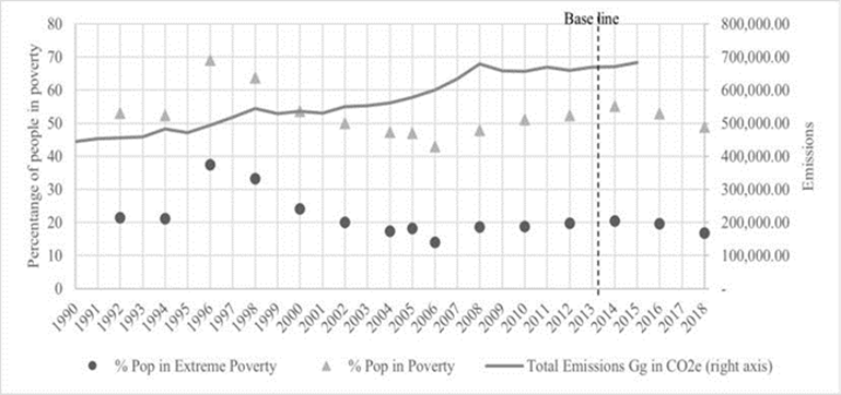
So far, the sixth communication of climate change (INECC, 2018) states that the direct GHG emissions in the country have reached 683 thousand (K) Gg of CO2 equivalent (GgCO2e), while the pursued goal of the fifth communication (SEMARNAT-INECC, 2012) was a decrease from 664K to 339K GgCO2e. The sixth communication establishes a new commitment: a 22% decrease of GHGs by 2030, compared to the level of 2013 (668K to 521K) if Mexico receives no international financial help to reduce emissions. If Mexico receives international financial help, such as tariff changes, carbon price adjustments, and the like, the conditioned measure would be a reduction of 36% (from 668K to 428K). This mismatch between the current policies and the reduction goal is alarming, as current policies, including the carbon tax, have had no effect on decreasing GHGs so far. In addition, this tax has been proven to be regressive, having negatively affected the welfare of the poorest households in the country (Chapa and Ortega, 2017a). Unfortunately, little has been advanced in the political discussion regarding how to jointly address the challenges on climate change and poverty (Middleton and O’Keefe, 2003), which directly and indirectly influence each other.
We understand that a successful tax policy should not only include the tax instrument and the characteristics of its implementation, but the rules for its revenue collection and spending. Regarding this, it is important to note that the carbon tax revenue is not allocated to climate change adaptation and mitigation measures such as subsidies, investment, and promotion of clean energy deployment or sustainable consumption practices; instead, the carbon tax is put in the same collection bag as any other tax of the Public Treasury. This, in addition to the unsuccessful collection of this tax by the government (SEGOB, 2013), greatly reduces the impact of the tax. Given that the tax was created to reduce gas emissions, Fiscal Law in Mexico could be reformed so that the tax would be used only as a revenue for investment in technology innovation, R&D, and green projects.2
In addition, based on the impact potential on other social variables by any tax policy scheme, the redesign of the carbon tax policy to achieve its main goal opens an opportunity to pursue additional social dividends through it.
Therefore, in the current research, we propose the use of a carbon tax applied to all sectors of the economy, subject to the constraint that the revenue is spent on sustainable development goals (SDGs) which are a priority for the current government and are related to poverty, education, and mortality. Thus, the reformed carbon tax would differ from the current tax in that it would be applied much more widely, and revenues from this tax would be used only to finance the achievement of other SDGs, and a tradeoff between the environmental SDGs would be balanced with a poverty SDG.
With respect to the 17 SDGs, preceded by the Millennium Development Goals (MDG), the effect that climate change has on them has not been calculated yet. In this paper, we focus our attention on three of them: SDG1 (poverty), SDG3 (child and maternal mortalities), and SDG4 (education). In the case of Mexico, previously, when MDGs were settled, the target was to reduce poverty by half by 2015, according to national measures, compared to the 1993 baseline. This implied going from 21.17% to 10.58% of the population living in poverty, which was not achieved. In this regard, Figure 1 shows that both poverty and extreme poverty3 levels increased from 2006 to 2014, and start slightly decreasing from 2014 to 2018, which coincides with the implementation of the carbon tax in 2014. Regarding the SDG3, maternal mortality, i.e., deaths for every 100,000 births, fell from 0.460 to 0.330 in 2008-2018 (the target for 2015 was 0.22); whereas child mortality, i.e., deaths for every 1000 births, dropped from 0.169 to 0.135 in the same period (the target for 2015 was 0.15).
The synergies and trade-offs between climate policy and the achievement of the SDGs are widely recognized -see, e.g., Gomez-Echeverri (2018), Sánchez et al. (2018), Sánchez (2018) and von Stechow et al. (2016). For instance, on the one hand, controlling climate change could help the poor avoid diminishing crop yields, winter mortality, and disaster-related losses; but it could also hurt the poor through regressive policies. On the other hand, escaping poverty implies households with better education and better income, which could lead to conservative consumption practices (benefitting the fight against climate change) and higher energy consumption (generating more GHG emissions). Despite the general insights on coordination that can be found in the literature (Szabo et al., 2016), an assessment of the impact of climate policy instruments, such as the carbon tax, on the SDGs has received much less attention (Campagnolo and Davide, 2019; Obergassel et al., 2017; Whalley, 1999).
In particular, Hurtado and La Hoz (2017) proposed a general framework of climate policy and SDGs interactions and applied it to Mexico. They found three key challenges: overcoming fossil fuel dependency, balancing rural and urban development, and developing an integrated implementation of social and climate policies. Villanueva (2017) analyzed the political context of SDGs in the country. She identified needed governance actions to allow SDGs fulfillment such as ensuring law enforcement, fighting corruption, and improving accountability, which are also fundamental to achieve climate commitments. Nonetheless, quantitative studies are needed to identify specific climate policy measures with the highest effect on improving the coordination of SDGs and climate actions.
The present paper contributes to fill this gap by evaluating the contrast between the currently failed specifications of the carbon tax policy and those that would have been necessary to achieve its main purpose and by analyzing additional dividends that such a tax could contribute towards the 2030 targets of three SDGs: poverty (SDG1), child and maternal mortality (SDG3) and education (SDG4). In addition, it examines whether the carbon tax is a viable policy instrument for enabling climate and SDGs policies coordination. To do so, we use a computable general equilibrium (CGE) approach, which is a suitable and broadly used methodology for quantitative policy impact evaluation (Allen et al., 2017; Bergman, 2005; Fossati and Wiegard, 2003). Specifically, we selected the Maquette for MDG Simulations CGE model (MAMS model, see section 2.1), developed by The World Bank, for its theoretical foundations, its policy-relevant flexibility, its sectoral detail, and its focus on SDGs (Lofgren and Díaz-Bonilla, 2010). To the best of our knowledge, this study constitutes the first application of the MAMS model to climate policy.
We found over 70 CGE studies applied to Mexico since the 1970s. However, a large share of them have focused on the role of specific sectors, such as tourism and agriculture, e.g., Kehoe and Serra-Puche (1986) and Yúnez-Naude (1992); or trade, e.g., Hinojosa-Ojeda and Robinson (1991) and Sobarzo (1994); environment-focused and SDG-related CGE studies only started gaining relevance since the mid-2000.
On the one hand, most environmental studies have targeted the effect of energy and climate policy, prices, and infrastructure on economic growth, climate change, and society. They have consistently found that increases in energy prices due to policy measures -such as the removal of subsidies (Rodríguez, 2003), the imposition of fossil taxes (Núñez-Rodríguez, 2015; Bravo et al., 2013), alternative technology promotion through subsidies (Elizondo and Boyd, 2017), and price liberalization (Brito and Rosellón, 2005; Moshiri and Martinez Santillan, 2018)- would negatively affect Mexican households, especially, low-income families. Nevertheless, conclusions regarding economic growth are disparate, i.e., while some found a growth path through increases in government revenue and investment (Brito and Rosellón, 2005; Rodríguez, 2003), others found significant contractions through induced effects across the economy (Alarco Tosoni, 2009; Núñez-Rodríguez, 2015). Furthermore, Boyd and Ibarrarán have concluded in several works (Boyd and Ibarrarán, 2002, 2011; Ibarrarán, 2001; Ibarrarán et al., 2011) that the fulfillment of climate change commitments would unlikely lead to a triple dividend with respect to social welfare increase, GHG emission reduction, and economic growth - a conclusion also supported by Castillo and Bravo (2010) and Hernández Solano and Yunez Naude (2016). Moreover, these authors have also estimated significant negative effects of climate change-related natural phenomena on society and the economy (Boyd and Ibarrarán, 2009; Ibarrarán et al., 2010; Ibarraran and Ruth, 2009). In contrast to these latter studies and Chapa and Ortega (2017a), Landa Rivera et al. (2016) found that there could be a triple dividend of the carbon tax if its revenues were redistributed in an appropriate and fully enforced manner, which has been proven difficult in practice.
On the other hand, few SDG-related CGE studies have focused on poverty (Beltrán, 2015; Vargas Hernández and Muñoz Jumilla, 2018) and universal social health insurance (Antón et al., 2016). Beltrán (2015) found that reforms on value-added tax and the direct income tax would modestly improve the income of low-income households, though without improving education, food security, and health; while the removal of the OPORTUNIDADES “cash transfer” program would significantly hurt the poor and extremely poor population. Vargas Hernández and Muñoz Jumilla (2018) concluded that economic liberalization in the State of Mexico would lead to better income distribution and lower poverty levels even though inequality would likely rise. Antón et al. (2016) found universal health insurance in the country could be feasible, and that the reallocation of government revenue from energy subsidies to social health insurance represents a viable policy. In addition, there are two studies with a specific focus on MDGs using the MAMS model (Ortega-Díaz and Székely-Pardo, 2008), which analyzed Mexico, and other Latin-American countries (Vos et al., 2008), pointed out that Mexico needed a 5% average growth rate and a 61% increase in net investment in public health infrastructure in the period 2003-2015 to reach MDGs targets altogether; while Ortega (2016) found that after the 2008 crisis the only feasible scenario route for Mexico to achieve the MDGs involves a combination of policy measures such as domestic debt and taxes.
The rest of the paper is organized as follows: The next section explains the specific characteristics of the CGE-MAMS model application, methods, and data collection and handling. Section 3 describes the base scenario and the construction of the alternative tax scenarios. Then, in section 4, we present and discuss the model simulation results. Finally, section 5 includes concluding remarks and policy implications of the study.
2. Methods and data
This section describes the selected computable general equilibrium model for the study, i.e., Maquette for MDG Simulations CGE model (MAMS model, section 2.1) and the characteristics of base data (section 2.2).
2.1 The MAMS computable general equilibrium model
The MAMS is a top-down, macro, country-level, recursive-dynamic CGE model for evaluating policy strategies aimed at reaching SDGs for low to medium-income economies (Lofgren and Díaz-Bonilla, 2010; Lofgren et al., 2013), built in GAMS software. It helps identify the most suitable and least costly policy among fiscal, internal, and external debts, and donations (Vos et al., 2008). So far, the model has been applied to over 40 countries since 2004, while only a few other models specifically designed for the evaluation of SDGs achievement can be found in literature, e.g., Campagnolo et al. (2018). Despite the fact that the MAMS model does not cover all 17 SDGs (it only covers SDGs 1,3,4, and 6, related to specific targets of poverty, maternal and child mortality, education, potable water, and sewage, respectively), it is unlikely that any model could include all SDG-relevant variables of interest within an integrated modeling framework (Allen et al., 2016).
The model quantifies the economy-wide effects of reaching each of the above-mentioned SDGs through either public or private expenditure as well as spillover and crossover effects throughout the economy. In addition, it considers whether the government budget comes from taxes and if those taxes are related to household income or collected from enterprises to incentivize carbon emissions reductions. Therefore, the MAMS is able to analyze any trade-off between reaching SDGs and the effects on the economy if the budget assigned to reaching the SDGs comes from taxes. Once we have a general equilibrium solution for reaching SDGs, the taxes are related outside the model with the elasticity of carbon emissions for each economic activity. Because of these characteristics, it constitutes the best option for the proposed study.
The MAMS model includes three modules: the static equilibrium, the dynamic equilibrium, and the SDGs module. A complete description of the MAMS model can be found in early studies of Bourguignon et al., 2008, then in Lofgren and Díaz-Bonilla (2010), and more recently in Lofgren et al. (2013). It is summarized in Figure 2.
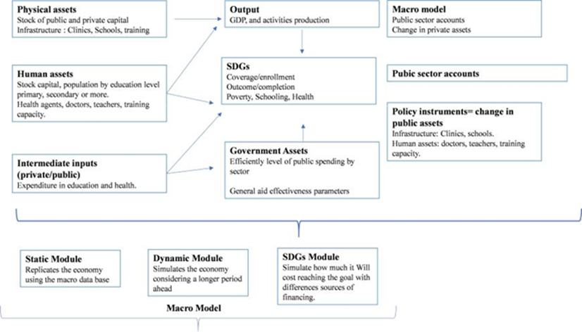
Source: Authors’ elaboration based on Bourguignon et al. (2008) and Lofgren et al. (2013).
Figure 2 MAMS model modules
The first module handles the set of equations that describe the economic relationships required for equilibrium. From an extensive data set -which consists of a Social Account Matrix (SAM), the rates of growth of several economic variables, their elasticities, prices, population and other socioeconomic indicators (see section 2.2)- the MAMS model simulates production and price decisions; households and government consumption; private and public investment; national and foreign trade; income and expenditure of the government; and macroeconomic balances (i.e., government balances, external balance of payments, saving and investment balances, and inputs markets).
The second module updates the parameters estimated in the base year using growth rates of the social and economic variables that are considered exogenous, e.g., population growth, government expenditure, government consumption, etc. In this regard, the model allows the use of average growth rates during the whole period of simulation, or different rates by subperiods, to define the growth trajectories of exogenous variables.
The third module estimates the path of SDG-related indicators under the considered assumptions, taking into account production activities and structural economic characteristics that are related to the achievement of SDGs, for example, health provision, education services, and the size of the labor force by type (unskilled, semi-skilled and skilled). Specifically, the achievement of each of the SDG targets is set as a “production function” with inputs at the aggregate level of the MAMS database (Lofgren et al., 2013). In this module, the settings of proposed carbon tax-rate scenarios (see section 3.2) are simulated to determine whether it is possible to achieve SDGs targets. Note that, while trends of SDG3 and SDG4-related indicators are an output of the MAMS simulations, SDG1-related indicators are obtained outside the MAMS through household welfare calculations, based on simulated household conditions and national household survey data.
In summary, the model includes the macroeconomic processes, the public policy decision of the government (GOV), the saving and investment decisions of the households (HH), the effects from the rest of the world (ROW), and the skill levels of workers according to their years of schooling. The model assumes the following statements: perfect market competition, economic actors are price takers, markets clear according to Walras law (supply is equal to demand), domestic trade versus international trade of goods and services uses Armington elasticities, household consumption uses linear expenditure system (LES) elasticities. Each period markets are in equilibrium taking into account prices, production, consumption, income, and expenditures of the institutions.4 The macroeconomic balances use macro closures which in the case of Mexico for the base scenario are: 1) GOV closure with fixed tax rate, flexible savings, flexible domestic debt, fixed foreign debt; 2) ROW closure with flexible exchange rate, fixed external debt; 3) investment-saving: closure with fixed private investment absorption, flexible total investment, flexible savings rate. When we incorporate the simulations, we make the policy tool flexible: tax, foreign debt, or domestic debt.
According to Lofgren and Díaz-Bonilla (2010), factor markets with endogenous unemployment are assumed in the MAMS model. The supply curve is upward-sloping, and it turns vertical when the market reaches full employment (the minimum unemployment rate is reached). When the factor market is below full employment, the unemployment rate is the clearing variable; at full employment, the economy-wide wage clears the market. The unemployment represents the degree of underutilization of the factor.
2.2 Data handling
Of the large data set required by the MAMS model, the social accounting matrix (SAM) is the central point. This matrix describes an extended input-output accounting system that includes bidirectional transactions among all producing and non-producing sectors in the economy, such as industries, primary factors and institutions (Breisinger et al., 2009; Thorbecke, 2017). It is a square matrix that reflects the circular flow of income of an economy in a specific year; and it contains the income-expenditure flows between households, enterprises, government, and the rest of the world. The SAM satisfies the macroeconomic identity that saving equals investment, representing a general equilibrium of the economy in a point of time, therefore it is used for calibrating general equilibrium models. In the SAM, each account is represented by a column and a row. The columns contain the expenditures and the rows the incomes. For each account, its total income must equal its total expenditure (see Table 1).
Table 1 Aggregated SAM - Mexico 2008
| EA | FG | LAB | H | GOV | ROW | TAX | Mtar | INT | S-C | INV | dstk | Total | |
|---|---|---|---|---|---|---|---|---|---|---|---|---|---|
| EA | 18,194,870 | 18,194,870 | |||||||||||
| FG | 6,253,671 | 7,313,116 | 1,546,108 | 2,205,154 | 3,243,670 | -76,026 | 20,485,693 | ||||||
| LAB | 3,411,296 | 3,411,296 | |||||||||||
| H | 3,411,296 | 221,766 | 291,336 | 97,573 | 7,185,007 | 11,206,978 | |||||||
| GOV | 304,914 | 213,604 | 1,238,984 | 35,783 | 1,275,005 | 3,068,290 | |||||||
| ROW | 2,266,453 | 440,514 | 127,126 | 84,146 | 2,918,239 | ||||||||
| TAX | 69,891 | 1,169,092 | 1,238,984 | ||||||||||
| Mtar | 24,369 | 11,414 | 35,783 | ||||||||||
| INT | 65,301 | 116,418 | 181,718 | ||||||||||
| S-C | 8,460,012 | 1,902,627 | 1,056,872 | 208,144 | 3,441,089 | 15,068,745 | |||||||
| INV | 3,243,670 | 3,243,670 | |||||||||||
| dstk | -76,026 | -76,026 |
Source: Own elaboration.
For this study, we adapted the 2008 SAM of Chapa and Ortega (2017b) to comply better with the MAMS modeling framework. This SAM was built using national input-output tables (INEGI, 2014), aggregated to the 37 activities of the 2013 World Input-Output Database (WIOD) of sectoral CO2 emissions (WIOD, 2016); and other socio-economic data from Mexican official databases (INEGI, 2016). We also take into account the latest statistics and reduced expected GDP growth rates in response to the pandemic situation. Appendix A describes in detail the SAM classification and data handling.
The adjusted SAM in this study consists of 12 aggregated accounts (Table 1): 40 economic sectors (EA); 40 goods and services (FG); 3 types of labor, classified according to their schooling level (LAB); 8 categories of households (H), i.e., extreme or food poor, capabilities poor, patrimony poor, and rural and urban non-poor; a government institution (GOV); the rest of the world (ROW); net taxes, import tariffs and interests (TAX, Mtar and INT); public and private saving-capital accounts (S-C); public and private investment (INV); and changes in inventories and statistical differences (dstk).
Although a SAM can be constructed for a more recent year, the last official input-output matrix of Mexico is the one of 2013, as there exists evidence indicating that the Mexican economy has not presented a strong structural change during the 2003-2013 period. For example, Beltrán et al., 2017), through the use of linear multipliers based on Social Accounting Matrices, concluded that between 2003 and 2012, the economy of Mexico did not change significantly. Like-wise, in order to support the use of the 2008 SAM, a structural change analysis was carried out comparing the classification of economic sectors by their backward and forward linkages (generally dependent, dependent on interindustry demand, dependent on interindustry supply, and generally independent) of the years 2008 and 2013 for two levels of disaggregation: 37 sectors according to the Nomenclature Statistique des Activités Economiques dans la Communauté Européenne (NACE) and 79 subsectors according to the North American Industry Classification System (NAICS). They found that between 70% and 80% of the economic sectors maintain their classification in both years.5
Other socio-economic parameters that are required by the MAMS model were compiled from several national and international databases of reliable institutions. For example, “Growth in real GDP at factor cost by year” data were obtained from the National Center for Macroeconomic Analysis; “Annual growth rate for world price of exports” data, from the Organization for Economic Cooperation and Development; and “Number of enrolled in cycle c by year” data, from the Ministry of Education. The description and source of all parameters are described in Appendix B.
3. Scenario setting
We simulate three scenarios for the period 2008-2030. Both IPCC and SDGs have 2030 as their target year: the 2030 IPCC target due in 2030 is to reduce greenhouse gas emissions by 22% of greenhouse gas emissions, and the SDGs targets can be seen in Table 2 below. The first scenario is the base case scenario (section 3.1), which estimates the path of the economy by calibrating market-clearing economic growth rates under the original 2008 tax scheme and ceteris paribus economic conditions; and two other scenarios (section 3.2), which consider an escalated direct tax on activities to calculate the required tax rate for market clearing and for potentially reaching SDG3 and SDG4, and the effect on SDG1 (child and maternal mortality, education and poverty, respectively).
Table 2 Trends and targets of SDG-related indicators
| Target 2030 | 2008 | 2018 | Status in | Target |
| 2018 | 2030 | |||
| SDG1.2 Reduce at least by half the proportion of men, women and children of all ages living in poverty in all its dimensions according to national definitions (MDG1). | 0.186 | 0.168 | On the way | 0.1095 |
| SDG3.1 Reduce the global maternal mortality ratio to less than 70 deaths per 100,000 live births. The original goal of MDG5 is to be reduced it by 3/4. | 0.46 | 0.33 | Far | 0.223 |
| SDG3.2 End preventable deaths of new-borns and children under 5 years of age, with all countries aiming to reduce neonatal mortality to at least as low as 12 per 1,000 live births and under-5 mortality to at least as low as 25 per 1,000 live births. MDG4 used to be the reduction of child mortality in 2/3 in children below 5 years old. But the population council (CONAPO) predicted 12.8%. | 0.169 | 0.134 | On the way | 0.128 |
| SDG4.1 Ensure that all girls and boys complete free, equitable and quality primary and secondary education leading to relevant and effective learning outcomes (MDG2). | 0.918 | 0.976 | Almost reached | 1.000 |
Source: Own elaboration.
3.1 Base case scenario
Mexico has already reached the SDG1 target of reducing extreme poverty ($1USD PPP) by half. Nevertheless, it has yet to eradicate extreme poverty and achieve the national target on poverty alleviation of 10.95%. Regarding the latter, poverty according to national measures is expected to drop from 16.8% in 2018 to 10.95% in 2030, giving the impression that the goal is feasible to be reached. On the other hand, in 2018, maternal mortality (SDG3.1) is still far from the target, while child mortality (SDG3.2) is on its way, as can be seen in Table 2. We model both SDG3 targets together as they are part of the same objective. Finally, the target on terminal efficiency in primary school is on its way, though it is difficult to ever achieve 100% as there are always dropouts and grade repeaters. The education received by students influences the types of workers in the labor market as the labor force is simulated considering the following simulated behavior: some students start primary school at the age of 6, others start later, some of them pass, others fail, some drop-out, some repeat a grade and others enter the labor market. Then, the endowment of workers of skill-type lab in time t equals the sum: [non-retired type lab of previous year (t-1)]+[entrants of type lab graduated from different school grades in t-1]+[entrants type lab from drop-out in each school grade in t-1]+[entrants type lab out of the school system (especially 12-year olds)], see Lofgren et al. (2013).
On the one hand, it is recognized that the achievement of these health and education-related targets require high levels of financing (Ortega Diaz, 2016; Vos et al., 2008). Thus, new policies are necessary to reach SDGs following the 2020 health crisis particularly since actual GDP growth rates from 2019 to 2020 were negative and average growth rates afterwards were below 1% per year. Consequently, most SDG-related indicators cannot be reached with the current economic trend (Table 2).
On the other hand, as explained above, the carbon tax implemented in Mexico since 2014 is equivalent to a tax rate of 0.03% on mining and quarrying (EA2) through taxing carbon, and of 0.5% on “coke, refined petroleum, and nuclear fuel” (EA12) through taxing gasoline, diesel, jet fuel and coke (Chapa and Ortega, 2017a). Chapa and Ortega (2017b) have suggested that the carbon tax imposed only on EA2 and EA12 is not enough to reduce emissions as other important emitters including construction (EA6), “electricity, gas and water supply” (EA3-EA5), “inland transport” (EA24) and “food, beverages and tobacco” (EA7) do not face the carbon tax. The fact that spending of this tax revenue is not linked to climate change further reduces its impact, as we noted earlier.
Linking both of these targets is the aim of the current research. Therefore, to analyze whether the original tax scheme conditions would have sufficed for achieving SDG targets, the base case scenario does not include the carbon tax, just the current direct tax for activities (i.e., an average direct tax of 0.068% for EA2 and 1.013% for EA12). Increasing this activity tax by 0.03% or 0.5% does not produce enough revenue to achieve the other goals (poverty, education, mortality), the achievement of the goals comes with an optimization of the model where the production tax for all production activities is scaled up. This analysis aims to simulate what level of tax would achieve the goals and decrease greenhouse gas emissions as well.
The tax scenarios that are needed to reach the SDGs targets are described in the next section, the resulting level of taxes would then be compared to the current carbon tax to discover a trade-off or synergy between SDGs and greenhouse gas emissions policies.
3.2 Tax scenarios
We are using the standard model by Lofgren et al. (2013). In this model, markets have the same set of factors, quantities demanded and supplied are set equal, and each market clears by its factor-specific wage variable, for each activity, and time-specific wage differential, considering a fixed unemployment rate.
Within the general equilibrium model, the tax simulation is carried out by solving the following balancing equations of government income (equation 1) and expenditure (equations 2 and 3) see Lofgren et al. (2013):
where: Y G=government income; T I N Si,t=direct tax rate on the non-government institutions i; Y Ii,t=income from the non-government institutions; tff ,t=direct tax on the factor f ; Y Ff ,t=income from factor f ; taa,t=tax rate on activity a; P Aa,t=price of activity a (grow Unitarian income); QAa,t=quantity (level) of the activity; tvaa,t=VAT on activity a; P V Aa,t=Price of VAT (factors income by unit of activity a; QV Aa,t=quantity of aggregate value; tmc,t=tax rate on imports; pwmc,t=price of imports of c (UME); QMc,t=quantity of imports of product c; tec,t =tax rate on exports; P W Ec,t=world price of exports of c (UME); QEc,t=exported quantity of product c; E X Rt=Exchange rate (domestic currency by UME); tqc,t=tax rate of sales; P Qc,t=Price of composite product; QQc,t=quantity of product c provided to domestic market (composite offer); Y I Fgov,f ,t=income of factor f for the domestic institution i; T RI Igov,i,t=transferences from institution i0 to i (both in the set INSDNG); and transf rgov,row,t =per capita transfers of institution i0 to household i, set for t in T .
Particularly, taa,t is the tool used to increase the government income by taxing all activities, and to find the required tax to reach the SDG targets. This additional income is allocated to increasing government spending directly in activities of health services for SDG3 and education for SDG4, and investing in education or health public infrastructure (equation 2) through construction activities, and in other activities that contribute to reaching SDG targets based on cost effectiveness analysis (equation 3, see Appendix C).
The real government consumption of infrastructure services, which is determinant for mitigating mortality and increasing schooling, is determined by the following equation:
where QGc,t = quantity consumed by the government of product c; QF I N Si,f ,t=real endowment of factor f of the institution i; and igfc,f ,t =quantity consumed by the government by unit of infrastructure capital stock f . Moreover, the real consumption of government (excluding infrastructure services) is:
where QGGRW t=real consumption government growth of c in relative to t−1; qg01c,c0 ,t=government consumption quantity by unit of capital stock different from infrastructure f ; and QGGRW Cc0,t=real government consumption growth of c in t relative to t − 1. Once the tax is collected, the decision of which sectors its revenue should be spent is determined so that the markets are in equilibrium every year.
These scenarios simulate how implementation of alternative tax rates affects economic growth and the SDG, via the revenue allocated to public infrastructure investment in health (scenario SDG3-tax) or education (scenario SDG4-tax). Once SDG-related indicators are close to achieving the committed targets by 2030, and the economy is in equilibrium, the resulting tax rate and the production activities in the economy are used considering the production elasticity of carbon emissions and quantify how much the current carbon tax should be increased to reach the SDGs and the resulting impact on production of greenhouse gas emissions.
4. Results and discussion
Figure 3 shows the tax rate that is required for the achievement of SDG targets under equilibrium for each scenario. The results show that the tax on production, of the base case scenario, would never have sufficed to achieve any of the SDG (see Figure 4). In other words, the level of tax revenue needed to clear the government budget and come closer to reaching SDG targets would need to be much higher than the actual tax imposed. Specifically, scenario SDG3AB-tax estimates a tax rate of 7.7% by 2019; and due to the pandemic situation, it would need to be increased to 14%, and then stay steady at around 15% until the goals are reached in 2030. While scenario SDG4-tax estimates a rate of 12.1% by 2024, and starts decreasing from 2025 (when the last primary school generation enrolls and achieves terminal efficiency in 2030).
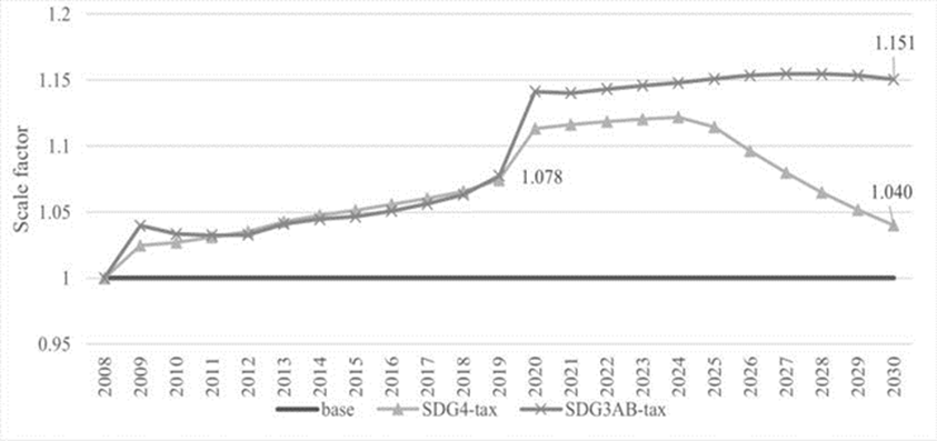
Source: Authors’ calculations from the CGE model.
Figure 3 Activities tax rate - scaling factor for all direct and indirect taxes
Note: SDG4-tax implies that all government revenue from tax is allocated to reach the SDG4 on education, and SDG3AB-tax allocates revenue both types of mortality.
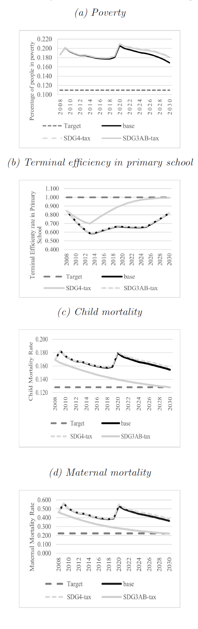
Source: Authors’ calculations from the CGE model.
Figure 4 Simulation of indicators related to SDG targets
These tax rates would lead to significant changes in government revenue and government consumption of goods and services allocated to reach the goals, including fixed investment, changes in assets, private transfers, domestic interest payments, and external debt payments. In the base scenario for the year 2030, the total government consumption in the base case scenario is 11.9% of GDP, while to achieve the SGD4s, total government consumption increases to 13.4% of GDP, and to 14.2% of GDP for SDG3. The country would achieve terminal efficiency (SDG4) if the tax is allocated to education activities and infrastructure, as can be seen in Figure 4b. Reaching the target on child mortality and maternal mortality is possible with higher taxes, which revenue is redirected to health services and hospital infrastructure (figures 4c and 4d). It should be noted that, none of the scenarios examined leads to achieving the SDG1.2 target on poverty (Figure 4a) which worsen under scenarios SDG3-tax and SDG4-tax, compared to the base scenario.
Table 3 shows the gap between the 2030 simulated scenarios and the 2030 base case scenario and is consistent with what we observed in figures 4a-d. The column with the scenario SDG3-tax describes the situation when the tax revenue is spent in decreasing both types of mortality; and it is found that, without taking action, the gap in 2030 would be 0.14 for SDG3.1 and 0.02 for SDG3.2; whereas using the revenue, both goals would be reached, and the gap would be zero.
Table 3 Gap from selected 2030 SDG targets
| Goal | GAP | Base case | SDG4-taxSDG3-tax | Actual gap by 2018a | |
| Poverty | SDG1 | 0.059 | 0.072 | 0.071 | 0.067 |
| Maternal mortality | SDG3.1 | 0.141 | 0.165 | -0.002 | 0.160 |
| Child mortality | SDG3.2 | 0.026 | 0.030 | 0.000 | 0.029 |
| Education | SDG4 | 0.182 | 0.007 | 0.182 | 0.346 |
Notes: a See table 2.
Source: Authors’ calculations from the CGE model.
However, there is no effect in this scenario for SDG1 and SDG4. On the other hand, scenario SDG4-tax, which implies spending the tax revenue in SDG4 only, succeeds in reaching almost 100% of terminal efficiency in primary school by 2030 with negligible gap of 0.007 percentage points. Both scenarios imply massive changes in government budget allocation to basic education services (which would almost double) and public education infrastructure (an up to 30% increase), or health infrastructure (a 61% increase over the whole period).
Interestingly, indicators related to target SDG1 had a more favorable trend under the base conditions than our analysis estimates. Particularly, targets SDG3.2 and SDG4.1 are virtually achieved by 2030 (Table 3). The latter suggests there were changes and spillover effects in the economic system that affected SDG1 indicators that were not captured in the simulations, such as, for example, income redistribution spillovers and non-governmental education programs.
Notably, mortality (SDG1) is significantly affected by the tax we have been examining due to its distortionary effects on household consumption and worker remuneration. The tax causes a decrease in the consumption of each household (Figure 5).
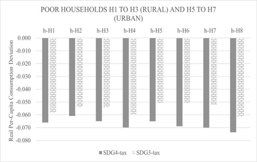
Note: Poor households correspond to H1 to H3 (rural) and H5 to H7 (urban).
Source: Authors’ own calculations using the CGE.
Figure 5 Household’s consumption deviation in 2030 from the base year
All households from both rural and urban areas decrease more their consumption under the scenario to achieve SDG3, than when SDG4 is pursued. This occurs because under SDG4 the surplus in government revenue goes to health services, while under SDG3 goes to education services, which allow students to reach higher levels of schooling and access better-paid jobs, and decreases the impact on poverty. However, this rebound effect is not enough to reach SDG1. Another important finding is that the tax that is spent on SDG4 and SDG3 seems to be progressive because the consumption of poor house-holds (H1-H3 and H5-H8) decreases less than non-poor households (H4 and H8).
The data of Figure 6 compares the consumption trends of the poorest households with the non-poor households in both urban and rural areas. Even when the tax is imposed across all economic activities using the same scaling factor, the tax affects each household type’s consumption patterns differently, with the tax devoted to SDG3 being less beneficial to consumption.
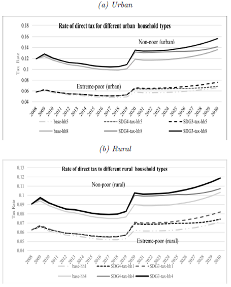
Source: Authors’ own calculations using the CGE.
Figure 6 Rate of direct tax for different household types
Furthermore, a carbon tax on all activities negatively affects trade by decreasing imports, exports, and investment, as well as GDP (see Table 4). The increased tax burden in scenario SDG3-tax would cause a reduction in private consumption by 2030 of -1.3%, compared to the base case scenario. In turn, this lower GDP would lead to falling wages, production, and capital. Accordingly, the simulation results for these two scenarios show that consumption would only increase for the government, which is coherent with the proposed fiscal policy of expenditure on public education and health services and infras-tructure.
Table 4 Macro indicators in year 2008 in column 2 and by simulation in final year (2030) in other columns
| Indicator | 2008 | Final year (2030) | Deviation from base case | |||
| Base | SDG4-tax | SDG3-tax | SDG4-tax | SDG3-tax | ||
| Absorption (Total Nominal LCU) | 1,203 | 1,725 | 1,618 | 1,650 | -0.062 | -0.043 |
| Real household consumption per capita | ||||||
| h-H1 | 1.39 | 1.29 | 1.21 | 1.21 | -0.066 | -0.058 |
| h-H2 | 2.17 | 2.23 | 2.10 | 2.11 | -0.061 | -0.054 |
| h-H3 | 2.96 | 3.18 | 2.97 | 3.01 | -0.065 | -0.054 |
| h-H4 | 8.10 | 8.37 | 7.78 | 7.87 | -0.07 | -0.06 |
| h-H5 | 1.93 | 2.08 | 1.94 | 1.97 | -0.065 | -0.051 |
| h-H6 | 2.61 | 2.91 | 2.71 | 2.76 | -0.069 | -0.051 |
| h-H7 | 3.53 | 3.98 | 3.70 | 3.77 | -0.07 | -0.052 |
| h-H8 | 9.76 | 10.74 | 9.95 | 10.08 | -0.074 | -0.062 |
| Macro indicators by simulation and year (% of nominal GDP) | ||||||
| Absorption | 100.5 | 106.6 | 107.1 | 107.0 | 0.005 | 0.004 |
| Consumption - private | 61.1 | 61.6 | 61.8 | 60.8 | 0.004 | -0.013 |
| Consumption - government | 12.9 | 11.9 | 13.4 | 14.2 | 0.121 | 0.191 |
| Investment - private | 17.9 | 19.0 | 18.9 | 18.6 | -0.008 | -0.022 |
| Investment - government | 9.2 | 14.1 | 13.1 | 13.5 | -0.071 | -0.044 |
| Exports | 18.4 | 14.2 | 13.6 | 13.7 | -0.041 | -0.037 |
| Imports | -18.9 | -20.8 | -20.7 | -20.7 | -0.003 | -0.005 |
| GDP at market prices | 100.0 | 100.0 | 100.0 | 100.0 | 0.000 | 0.000 |
| Macro indicators by simulation and year (% of nominal GDP) | ||||||
| Net indirect taxes | 0.79 | 0.8 | 0.82 | 0.89 | 0.031 | 0.110 |
| GDP at factor cost | 99.2 | 99.2 | 99.2 | 99.1 | 0.000 | -0.001 |
| Foreign savings | 1.7 | 19.8 | 17.8 | 18.1 | -0.103 | -0.084 |
| Gross national savings | 24.7 | 26.5 | 24.8 | 25.0 | -0.063 | -0.055 |
| Gross domestic savings | 26 | 13.3 | 14.2 | 13.9 | 0.068 | 0.047 |
| Foreign government debt | 3.0 | 89.0 | 95.0 | 93.2 | 0.068 | 0.047 |
| Foreign private debt | 3.6 | 5.0 | 5.3 | 5.2 | 0.068 | 0.047 |
| Domestic government debt | 11.7 | -12.9 | -13.8 | -13.5 | 0.071 | 0.049 |
Source: Authors’ calculations from the CGE model.
4.1 Assessing impact of equilibrium tax on GHG emissions reductions
The lower GDP in SDG3-tax and SDG4-tax compared to the base case scenario imply a lower level of greenhouse gas emissions, triggered by reduced consumption and consequent decreases in production of main emitters and other sectors. Based on the emissions-GDP elasticity calculated by Conte Grand and D’Elia (2013),6 total GHG emissions in equivalent CO2 by 2030 would have been lower by 5.65% for SDG4-tax and 4.00% for the SDG3-tax, compared to the base case scenario. In absolute terms, this would have represented reductions of 39,002 and 27,606 GgCO2e, respectively.7 However, the reduction in CO2 emissions under any of the scenarios we examined is very far from what is required to fulfill the countrys climate commitments. For example, in order to fulfill The Paris Agreement requirements, Mexico must achieve a 22 percent reduction of GHG emissions by 2030, which is equal to 168,017 GgCO2e.
These estimations must be taken with caution, as they are approximations. The implementation of a carbon tax rate of 15% could cause a structural change in the long-term relationship of GDP and emissions, changing the GDP elasticity of emissions.
5. Conclusions
This paper analyses the suitability of the carbon tax as a stand-alone tool to help achieve SDGs targets while decreasing carbon emissions. To do so, we perform a scenario simulation analysis with the MAMS general equilibrium model, which allowed us to estimate the poten-tial of the proposed climate policy tool for the achievement of SDGs.
Particularly, we focused on the SDG1 (poverty), SDG3 (child and maternal mortality), and SDG4 (primary school terminal efficiency). In contrast to the actual carbon tax policy in the country, the proposed tax is imposed on all economic activities and its revenue is allocated differently in the simulations, i.e., either allocated to public health services and infrastructure, related to target SDG3, and services and public infrastructure of basic education, related to target SDG4.
We found that the carbon tax rate that would produce sufficient government revenue to approach SDG3 or SDG4 targets should be around 15%. This rate is 30 times higher, compared with the actual official carbon tax rate (0.5%), and would be almost like the current VAT of 16%. In this regard, household welfare is likely to be significantly affected, especially for the poor, which would effectively offset any poverty alleviation efforts in the country (related to SDG1).
Given that most of the decrease in household disposable income comes from consumption and not from savings and investment, economic principles indicate that the direct tax alternative would be less distortionary than domestic government borrowing for long-run growth in GDP and private final demand. However, in practice, the alternative of combining increasing direct taxes with domestic debt is less distortionary and more feasible than raising taxes to 15% rates.
We conclude that the carbon tax, at least under its existing implementation scheme, is not a viable standalone policy tool to achieve both SDGs and climate change targets. Instead, attaining the coordination between climate and SDG-related efforts requires a basket of policy tools, which should include, for example, not only taxes but also debt; a carbon tax with different collection and revenue allocation standards, such as those proposed by Landa Rivera et al. (2016); and green funds that help shift the production to less polluting technologies with less negative effects on households.
Finally, these conclusions are aligned with previous studies that found some climate policy instruments to be unsuitable to achieve a double or triple dividend (for example, studies by Chapa and Ortega, and Boyd and Ibarrarán). They also coincide with the findings of the two SDG-related studies for the country, which point out the need for a radical change in the economic trajectory of the country to overcome major development challenges. Still, further quantitative research is needed to help identify which instruments may be optimal for a win-win situation between SDGs and climate policy.

