


 nova página do texto(beta)
 Inglês (pdf)
 Artigo em XML
 Referências do artigo
 Enviar este artigo por email
 Citado por SciELO
  Similares em
SciELO
Similares em
SciELO 
 Permalink
1. Introduction
The aim of this research is to analyse the association between knowledge and technical efficiency (TE) in small and medium-sized enterprises (SMEs) that belong to either manufacturing, trade, or service sectors in Mexico. Previous studies argue that firms typically deal with limitations that prevent them to use their inputs efficiently. Among others, different types of knowledge (e.g., human capital or innovation) determine how enterprises use scarce resources. Usually, such an association is intangible and, therefore, we are unable to observe and measure it directly. Under such circumstances, we aim to identify the knowledge- TE link in this article. By doing it, we contribute to the existing literature by i) providing empirical evidence on how different types of knowledge relates to TE in SMEs, and ii) providing policymakers with useful information about SMEs’ performance that can be used to inform the elaboration of policies aiming to attenuate harmful effects of the 2020 global economic recession. To accomplish these goals, this paper takes advantage of a firm-level dataset released by the National Institute of Statistics and Geography (Instituto Nacional de Estadística y Geografía, INEGI), which reports socio-economic data from 28 034 SMEs in the manufacturing, trade, and service sectors.1
The National Survey on Productivity and Competitiveness of Micro, Small and Medium Enterprises (Encuesta Nacional sobre Productividad y Competitividad de las Micro, Pequeñas y Medianas Empresas, ENAPROCE, published by INEGI) reports that there exist 111 958 SMEs in the manufacturing, trade, and service industries, which on average hired 3.22 million employees during 2017 (16% of the total employment in the three sectors).2 From the total number of workers in small and medium-sized firms, 20.9% and 18.0% have higher education, respectively. From the total number of small-sized firms, 24.4% indicate that the main obstacles for improving their market performance are: high taxes, expenses on paying taxes, paperwork needed to meet their obligations, lack of credit, and unfair competition with informal firms. Meanwhile, 92.4% use the Internet in their production processes. On the other hand, 74% of medium-sized firms train their workers, 40% have access to credit, and 98.4% use the Internet in production activities. Overall, SMEs in Mexico play an essential role in economic activity, especially in terms of employment. However, such enterprises deal with some limitations that might prevent them from reaching the maximum TE, that is, the maximum level of output that SMEs can reach if they use all inputs efficiently.
Among other things, surveyed SMEs in ENAPROCE report that the main obstacles for increasing their production and efficiency levels include: i) liquidity constraints for investing in research and development (R&D) activities, ii) lack of training for workers, iii) low-skilled labour and iv) complex tax liabilities (INEGI, 2015 and 2018). Such obstacles might influence their performance. Apart from the widely known inefficiency effects in the existing literature, economic theory and previous studies argue that different types of knowledge also influence firms’ performance, including the following: i) human capital or quality of labour (Admassie and Matambalya, 2002; Alvarez and Crespi, 2003; Taymaz, 2005; Charoenrat et al., 2013; Valderrama et al., 2015; Diaz et al., 2019); ii) innovations (Aw and Batra, 1998; Becchetti et al., 2003; Yang and Chen, 2009; iii) acquisition of licenses to use existing technologies (Becchetti et al., 2003; Taymaz, 2005); iv) creation of new technologies and transfers to other firms (Becchetti et al., 2003); and, v) managerial practices (Admassie and Matambalya, 2002; Taymaz, 2005). To better understand such a phenomenon, this paper examines the knowledge- TE link in SMEs.
Standard economic theory assumes that firms are fully efficient. This assumption seems to be unrealistic; therefore, the Stochastic Frontier Analysis (SFA) allows for technical inefficiencies (TI) in production activities. The SFA defines the production frontier as the maximum attainable output using a bundle of inputs efficiently. Input-output combinations bounded by the frontier represent the set of feasible outputs that can be produced using the existing technology. The SFA uses the Output-Oriented (OO) and the Input-Oriented (IO) methods to account for TI. The former suggests that, in the existence of TI, the firm can produce a higher level of output using the same amount of inputs. The latter approach states that, in the presence of TI, the firm can produce the same level of output using fewer inputs. Kumbhakar et al. (2015) show that the two approaches are similar and, with the correct reparameterization, lead to similar results.3 However, given the complexity in the estimation of the IO model, researchers prefer the OO model. So, following Kumbhakar et al. (2015) we use the OO single-step approach proposed by Wang (2002).
Using the single-step maximum likelihood method in Wang (2002), the OO approach estimates a production function and computes firm-specific technical (in)efficiency scores. Simultaneously, it hypothesises TI to be a linear function of inefficiency effects. By doing this, this study examines the impact of different types of knowledge on TI. The main findings suggest that the average technical efficiency (ATE) in the pooled sample is 54.6%. SMEs exhibit decreasing returns to scale (0.96). And SMEs with high-qualified workers, firms transferring their own technology to other firms less frequently, and those that use the Internet in their production processes tend to observe lower values of TI. In contrast, annual expenses on all procedures required to pay taxes enlarge TIs.
The structure of this paper is as follows. Section 2 includes an overview of the existing literature analysing TE in SMEs. Section 3 describes the SFA methodology, the set of variables in the production frontier and TI models. Section 4 presents the main findings and a brief discussion. Finally, section 5 concludes and provides a list of further steps.
2. An overview of previous studies
The existing literature uses either the parametric SFA, the non-parametric Data Envelopment Analysis (DEA), or both approaches to analyse firms’ performance. These methods compute strictly positive TE scores that can be used to assess the performance of enterprises. Murillo-Zamorano and Vega-Cervera (2001) present a comparison between the two approaches. The authors indicate that the main advantages of using the SFA are: i) the inclusion of random noise in the frontier function, which accounts for firm-specific short-term random shocks in the production process, and ii) its capability to accommodate skewness in the disturbance term. On the other hand, the attractiveness of the DEA comes from: i) their deterministic nature, it does not consider random noise, and therefore, ii) researches do not impose a specific functional form to the frontier function and to the statistical distribution of the inefficiency term. Murillo-Zamorano and Vega-Cervera (2001) and Murillo-Zamorano (2004) do not find evidence of strict superiority of one approach over the other.
Among other authors, Bojnec and Latruffe (2009), Bakucs et al. (2010), and Mamardashvili and Schmid (2013) argue that TE scores from DEA are remarkably sensitive to outliers and are usually smaller than SFA scores because the former approach considers all deviations from the frontier as inefficiencies. This seems to be an unrealistic assumption since the production activities are exposed to unexpected events, which should be accounted for in the production function. Furthermore, the DEA approach uses a two-step procedure to identify the efficiency effects. This is also true in some applications of the SFA method. Wang and Schmidt (2002) show that the two-step SFA approach leads to biased estimations and propose a single-step SFA model, which is particularly useful when researchers aim to identify the relationship between firm characteristics and efficiency levels. Including a random term in the estimation seems to be more consistent with real data, and a single-step procedure is more efficient than a two-step procedure. For these reasons, we use the single-step SFA approach in this analysis.
Aigner et al. (1977) and Meeusen and Van DenkBroeck (1977) introduce the SFA parametric approach into the economic literature. The SFA method is used to measure the performance of farms (Minviel and Latruffe, 2017), health institutions (Greene, 2004), manufacturing firms (Kathuria, 2001), universities (Stevens, 2005), and other entities. To refine the literature review, we focus our literature survey on those studies analysing TI in SMEs and on studies using Mexican firms as their main interest. Furthermore, given this investigation’s (empirical) nature, we look at the set of variables that influence TI scores. The first part of table 1 summarizes the existing studies examining TI in different industries worldwide. It shows that this literature mainly examines TI in developing countries using either a panel of firms or cross-sectional data. Apart from the set of widely known inefficiency effects in the SFA literature, for example, firm size, firm age, debts, exports, and regional effects, these studies include some indicators of knowledge in the TI equation (variables in bold in the last column of table 1). These indicators include R&D investments, technology transfers, innovation, extension services, human capital, and Information and Communication Technologies (ICT).
Table 1 An overview of empirical studies
| Study | Country | Period | Industry | Firms | Method | ATE | Inefficiency effects: variables in the TI equation (sign of the parameter in parentheses) |
| Other countries | |||||||
| Taymaz and Saatci (1997) | Turkey | 1987-1992 | Manufacturing firms | 513 firms (more than 25 employees) | SFA | Textile: 79.3%; cement: 83.7%; motor vehicles: 79.5%. | Number of employees (0-), regional to total output (0+), individually owned (0-), joint stock companies (-+0), shift-work (-+), subcontracting inputs (-), subcontracting outputs (0), advertising intensity (0+), communication intensity (0+), private domestic ownership (-), foreign ownership (-+), technology transfers from abroad (-) and time dummy variables |
| Zheng et al. (1998) | China | 1986-1990 | Manufacturing firms | 1,759 observations | DEA | Small: 78%; medium: 79%; large: 87% (75%-87% in 7 ind.) | Industry and time dummy variables (+-0), provinces dummies (+-0), productive labour to total employment (0), productive capital to total capital (+), share (+), responsibility (+), leasing contract (0), assets management (0), state-owned enterprises (+), collective-owned enterprises (+), large firm (-) and medium-sized firm (-) |
| Aw and Batra (1998) | Taiwan | 1986 | Manufacturing firms | 123,000 firms (exporters and non-exporters) | SFA | Textiles: 66.8% & 66.6%; clothing: 99.6% & 70%, paper and publishing: 62.7% & 68.8%; plastics: 69.4% & 69%; fabricated metals: 67.5% & 68.3%; iron and steel: 69.3% & 66.6%; machinery: 99.7% & 71.7%; electrical and electronics: 65.6% & 63.6% and transport equipment: 75.8% & 67.7%. | Utilisation rate (-0), age of the firm (-0), R&D and training (-0), foreign capital (0), interaction between R&D and training and foreign capital (-+0) |
| Bigsten et al. (2000) | Cameroon, Kenya, Ghana and Zimbabwe | 1992-1995 | Manufacturing firms | 960 observations | SFA | Cameroon: 39% (25%-67% in 4 ind.); Ghana: 27% (17%-36% in 4 ind.); Kenya: 22% (12%-35% in 4 ind.); Zimbabwe: 37% (30%-55% in 4 ind.) | Initial exporter (-), initial efficiency (-), continuous exporter (-), new entrant into exporting (-), country fixed effects (+-0), micro firm (0), medium firm (0), large firm (0), wood firm (-), textiles firm (-) and metals firm (-) |
| Lundvall and Battese (2000) | Kenya | 1993-1995 | Manufacturing firms | 235 firms | SFA | Micro: 60.5% (42%-76% in 4 ind.); small: 67.8% (53%-80% in 4 ind.); medium: 78.8% (77%-83% in 4 ind.); large: 83.5% (76%-90% in 4 ind.); very large: 87.8% (81%-93% in 4 ind.) | 1993 dummy (+-0), 1994 dummy (+-0), intermediate inputs (0), intermediate inputs square (+-0), age of the firm (+-), age square (+0) and intermediate inputs*age (-0) |
| Baek and Pagan (2002) | US | 1992-1998 | Standard and Poor’s ExecuComp | 1,030 firms (>20 employees) | SFA | Full sample: 78.74%. | Cash and non-cash base CEO’s salary (+), value of bonus (0), value of restricted stock granted (+), value of stock options granted (+), total CEO’s compensation (-), percentage of the company’s shares owned by the top manager (0) and years as a CEO (+) |
| Admassie and Matambalya (2002) | Tanzania | 1999 | Manufacturing and tourism firms | 148 SME firms | SFA | Pooled sample: 56%; textile: 71%; food: 47%; tourism: 47%. | Age of the firm (0+), age square (-0), size or number of workers (0+), acquisition of information technology (0), acquisition of IT square (0), skill intensity of labour (-+0), skill intensity of management staff (-0) and regional dummies (+-0) |
| Alvarez and Crespi (2003) | Chile | 1998 | Manufacturing firms | 157 micro, 796 small and 138 medium-sized firms | DEA | Micro: 67%; small: 61%; medium: 83% (34%-91% in 17 ind.) | Owner experience (0), owner’s education (+), variability of sales (0), human capital of workers (0), experience of workers (-), machinery age (+), equipment age (0), vehicles age (+), capital per worker (0), output sold in the domestic market (0), banking loan (0), output sold in the external market (0), technological development programme (0) and technical assistance funds (0) |
| Becchetti et al. (2003) | Italy | 1995-1997** | Manufacturing firms | 1,710 small firms (obs.) and 787 large firms (obs.) | SFA | Not reported. | Industry dummy variables (+-0), regional dummy variables (+), older 20% of sample firms (+), younger 20% of sample firms (+0), firms affiliated to groups (0), firms monitoring customer satisfaction (0), firms that created sale structures abroad (0), rents (+), interest payments (0-), degree of capacity utilisation (0), innovation or introduction of new products or processes (0), ICT investment per employee (-), software investment per employee (-), hardware investment per employee (0) and telecommunication investment per employee (+) |
| Söderbom and Teal (2004) | Ghana | 1991-1997 | Manufacturing firms | 143 firms (5 industries) | SFA | Full sample: 53% (from 2 to 841 employees) | Industry dummy variables (+-), regional dummy variables (0-), firm age (0), foreign ownership (0) and state ownership (0) |
| Taymaz (2005) | Turkey | 1987-1997 | Manufacturing firms | 12,788 small and large firms | SFA | Food and tobacco: 71.8%; textile: 73.8%; wood products: 72.1%; paper and printing: 83.1%; chemicals: 70.5%; glass and cement: 60.1%; basic metal: 65.6%; engineering: 72.2%; other manufacturing ind.: 40%. | Number of employees (0), regional to total output (0), individually owned (0), joint stock companies (0), shift-work (0), subcontracting inputs (0), subcontracting outputs (0), advertising intensity (0), private domestic ownership (-), foreign ownership (-), technology transfers from abroad (0), wage rate to account for quality of labour (-), women personnel (0), administrative personnel (0) and technical personnel (0)* |
| Yang and Chen (2007) | Taiwan | 2001 | Electronic firms | 7,122 SMEs and 468 Large firms | SFA | SMEs: 69.0% (64.8%-70.6% in 9 subsectors); large: 70.4% (64.9%-77.0% in 9 subsectors) | Firm age (-), welfare expenditure per employee (-), export intensity (-), R&D intensity (-), subcontractor or outsourcing (-), barriers to entry (+), regional R&D intensity (+), size of regional industry (-) and regional employment in Medium-sized firms (-) |
| Diaz and Sanchez (2008) | Spain | 1995-2001 | Manufacturing firms | 1,368 small firms and 530 large firms | SFA | Small: 83.4% (51-100 workers); large: 80.9% (>100 workers) | Ratio of temporary workers (+), foreign shareholders (-), market share (-), capital by worker (+), gross investment over capital (0), public limited company (-) and six size dummy variables (-) excluding the largest range (more than 500 workers) |
| Charoenrat et al. (2013) | Thailand | 2007 | Manufacturing firms | 56,441 SMEs | SFA | Pooled sample: 51%; small: 48%; medium: 67% (44%-63% in 7 subsectors). | Dummy variable for small firms (-), firm age (-), skilled labour to total labour (-), municipality dummy variable (-), dummy variable for Bangkok (-), regional dummy variables (-+0), dummy variable for individual proprietor (-), juristic partnership (-), limited liability company (-), state-owned firm (+) and cooperative firm (-) |
| Mexico | |||||||
| Hernandez-Trillo et al. (2005) | Mexico | 1997 | All sectors | 10,332 micro firms (up to 6 or 16 workers) | SFA | Not reported. | Professional occupation dummy (-), years in business (-), formal sector dummy (-), inherited business dummy (+), bank dummy (-), savings and loans dummy (-), friends/relatives dummy (-), money lenders dummy (-), previous job dummy (-), credit from suppliers/clients dummy (-) and female dummy (+) |
| Becerril et al. (2007) | Mexico | 1970-2003 | All sectors | 32 states | SFA | Pooled sample 1970-2003: 77.1% (40.7%-91.9%) | Linear time trend (-) and squared time trend (+) |
| Aguilar (2011) | Mexico | 2006-2008 | Manufacturing firms | 91 municipalities and 5 subsectors | SFA | Footwear: 77.3%; garment: 64.6%; wood products: 50.7%; textile: 30.6%. | Lineal time trend (+), industrial concentration (-), wage increments (+) and education (-) |
| Becerril et al. (2012) | Mexico | 2008 | All sectors | 19 two-NAICS digits sectors | DEA | 64.4% with constant | There is not a technical inefficiency equation returns to scale and 71.9% with variable returns to scale (20.9%-100% in 19 sectors) |
| Chavez and Fonseca (2012) | Mexico | 1988, 1993, 1998, 2003 & 2008 | Manufacturing firms | 32 states | SFA | 1988: 57.7%; 1993: 59.4%; 1998: 64.5%; 2003: 69.1%; 2008: 73.5% (50.6%-76.4% in 4 regions) | There is not a technical inefficiency equation |
| Herrera (2012) | Mexico | 2003-2007 | Manufacturing firms | 6,626 micro, small, medium and large-sized firms | DEA | Micro: 52%-93% (12 NAICS sectors); small: 48%-87% (21 NAICS sectors); medium: 54%-95% (20 NAICS sectors); large: 50%-96% (20 NAICS sectors) | There is not a technical inefficiency equation |
| Tovar (2012) | Mexico | 1988, 1993, 1998, 2003 and 2008 | Manufacturing firms | States (21 three-NAICS digits sectors) | DEA | High tech firms: 80-100% | Specialization index (-), Urbanization index (-) and TLCAN dummy (-) |
| Valderrama et al. (2015) | Mexico | 1985-2009 | Manufacturing subsectors | 25 manufacturing industries | SFA | 1985: 70.1%; 2009: 67% (59.7%-77.1% in the 1985-2009 period). | FDI to total domestic sales (+), human capital or labour productivity (-), capital or cost of capital (+), Lerner index (-) and time trend (0) |
| Morales (2016) | Mexico | 2006-2014 | Construction, trade, services and manufacturing firms | 853 formal and 5,553 informal micro- enterprises | SFA | Not reported. | Business time (-), formality (-), inherit the firm (+), gender-female (+), commercial bank credit (-), development bank credit (-), government credit (+), ‘caja popular’ (-), supplier credit (-), private lender (-), credit from fiends (-), empen˜o (-), clearing (-), savings (-), other source (-), business vision (-), training(-), expectations (-), previous experience(+) |
| Santos et al. (2019) | Mexico | 2004, 2009, 2014 | Automotive industry | Guanajuato and 15 states | DEA | 2004: 100%: 2009: 100%; 2014: 92.31% Guanajuato (77.24%-100% in other states) | There is not a technical inefficiency equation |
| Diaz et al. (2019) | Mexico | 1994, 1999, 2004 and 2009 | Automotive industry | 38 metropolitan areas and 34 municipalities | SFA | 52% in 1988 and 55% in 2008. South (20%-34%), centre-north (34%-40%), centre (59%-61%) and north (68%-86%) | Specialization index (-), schooling (-), linear time trend (-), squared time trend (+), assemblers dummy (+), centre-north dummy (-), north dummy (-), centre dummy (-), south dummy (omitted), TLCAN dummy (+) and metropolitan zone dummy (+) |
| Navarro et al. (2019) | Mexico | 2008-2015 | Electric sector | 13 divisions in the northern and Baja California regions | DEA | Baja California: 92.5% (65%-94.1% in other regions) | There is not a technical inefficiency equation |
| Borrayo et al. (2019) | Mexico | 1960-2013 | Manufacturing industries | 32 states | SFA | Not reported | Inistat (-) |
Notes: *Most of the subsectors show the indicated effect. NAICS: North American Industry Classification System (SCIAN in Spanish). Ind. stands for industries. + (-) indicates a positive (negative) effect of the corresponding explanatory variable on TI. Zero represents a non-statistically significant effect.
Source: Own elaboration based on the systematic literature review.
Previous studies encounter that increasing the ratio of R&D expenditures to total sales (R&D intensity) reduces or has no effect on technical inefficiency scores. The null effect of R&D activities on TI reveals that some SME firms cannot make large investments in innovation. Table 1 also shows that technology transfers (from abroad) have either a negative or a null effect on TI. The significance of such an effect may depend on how SMEs adapt new technologies to the current production processes. Furthermore, most of the parameter estimates suggest that the quality of labour (human capital) has a negative effect on TI. It implies that firms with high-qualified workers, including the manager, use available resources more efficiently.
Empirical evidence also suggests that investments in ICT increase or have no effect on TE. These investments facilitate communication within and between firms, and consequently, reduce inefficiencies. Regarding extension services (technical assistance) and investments in innovation, previous studies encounter a non-significant effect of these variables on firms’ performance. As in the R&D expenditures, SMEs may be allocating a limited amount of resources for training activities and innovation, which explains the insignificance of the corresponding parameters.
The second part of table 1 shows the set of studies looking at TE in Mexico. We encounter empirical research work for manufacturing, construction, trade, service, automotive and electric industries. Such investigations analyse either cross-sectional or panel data applying the two approaches, SFA and DEA. Previous studies in Mexico use either state, regional, municipality, sector or firm-level data. Becerril et al. (2007) use the SFA and encounter that TE in all sectors ranges between 40.7% and 91.9% in 1970-2003 (77.1% ATE) and Becerril et al. (2012) apply the DEA and find that TE ranges between 20.9% and 100% in all sectors in 2008 (64.4% and 71.9% ATE).
ATE scores go from 30.6% to 100% for manufacturing firms in Mexico. For example, Herrera (2012) estimates that ATE in 12-North American Industry Classification System (NAICS)4 digits micro, small, medium, and large manufacturing firms are 52%-93%, 48%-87%, 54%-95% and 50%-96%, respectively. Unfortunately, some authors do not report ATE in their studies and cannot be used for comparison (Hernandez-Trillo et al., 2005; Morales, 2016). The last column in table 1 shows the list of efficiency effects when authors estimate a TI equation. Although Aguilar (2011), Valderrama et al. (2015) and Diaz et al. (2019) use indicators of knowledge as inefficiency effects, for example, education or labour skills, this issue has been partially addressed in the existing literature in Mexico.
The existing literature includes some types of knowledge in analysing SMEs’ performance. Notwithstanding, there are still some questions that remain unanswered. Thus, the contribution of this paper is twofold. First, it provides empirical evidence on the knowledge- TE link in SMEs in Mexico using three different types of knowledge indicators in the TI equation (human capital, innovation, and technology transfers). Second, it provides policymakers with information about SMEs’ performance that can be used to design policies aiming to attenuate the harmful effects of the 2020 global economic recession.
3. Methods and materials
3.1 Method
This paper uses the OO approach of the SFA to investigate the influence of various types of knowledge on TE. Aigner et al. (1977) and Meeusen and Van den Broeck (1977) introduced this parametric approach in the economic literature to examine firms’ performance via TE. Among others, Kumbhakar (1987) defines the stochastic production frontier as the maximum attainable level of output that can be produced using the current technology and a certain amount of inputs. Standard economic theory assumes that firms are fully efficient and deviations from the frontier are attributable to random shocks. However, the SFA relaxes such an assumption by allowing for inefficiencies in the production process. Considering technical inefficiencies, the OO method defines the production frontier as follows:
where Y is total output, x is a vector of inputs, f (.) stands for the functional form of the frontier, and u is non-negative and measures TI. For small values of u, exp(-u)≅1-u. Thus, TE=exp(-u)=1-u=1-TI .
Previous studies applying the same methodology typically use the Cobb-Douglas (CD) and/or the TransLog (TL) functions to identify the frontier in equation (1). After taking the natural logarithm of equation (1), the CD function is given by the following expression:
where y
i
is the natural logarithm of total output of the i-th
firm, β
0=ln(A), β
j
are the parameters in the production function, x
ji
are the corresponding inputs in their logarithm forms, β
t
is the measure of technical change
where β
jk
=β
kj
the measure of technical change is equal to
For both equations, (2) and (3), v
i
is the random component which is assumed to be independent and
identically distributed (i.i.d.) with mean zero and constant variance,
To disentangle the composite error term and empirically compute the values of
u
i
, we assume a parametric distribution for the inefficiency term.
Empirical studies usually adopt either a half-normal
Assuming a truncated-normal distribution for u
i
, the SFA model uses the Jondrow’s (JLMS) formula (Jondrow et al., 1982) to obtain
where
where γ m are the parameter estimates of the (mean) TI equation. The marginal effect of the m-th inefficiency determinant on μ i is given by the following expression (Wang, 2002):
where Λi = μ i / σ u,i , it represents the ratio between the expected and the standard deviation of TI in firm i and is used as an argument of the standard normal and cumulative density functions, which produce the adjustment term in equation (6). The main advantage of Wang’s (2002) formulation is that these marginal effects are observation-specific.
3.2 Materials
The ENAPROCE collected firm-level data on 28 034 enterprises that hire between 11 and 250 workers in the manufacturing industry,7 and between 11 and 100 workers in the trade8 and service9 sectors.10 From the 28 034, 52% reported information about their economic activities in 2014 (INEGI, 2015), 48% in 2017 (INEGI, 2018), and 12 457 firms appeared in both surveys.11 Following Taymaz and Saatci (1997), Baek and Pagan (2002), Admassie and Matambalya (2002), and Taymaz (2005), the dependent variable in the frontier function is the value of total sales plus the change in stocks (output stock in January 1st minus output stock in December 31st) from all commodities produced in the corresponding firm.12 The total number of working hours hired in 2014 and 2017 measures the size of labour in the production function. To account for capital endowments, we use fixed-assets’ self-reported replacement value. The sum of annual expenses on raw materials, maquila, electricity, telecommunications, and other inputs represents the value of intermediate inputs. We also introduce a time indicator and 11- NAICS indicators in the set of estimations.
To guide the model specification of the TE equation, we use the previous empirical findings shown in table 1. Unfortunately, data availability prevents us from including all controls in the existing literature. We account for total firm’s expenses when it pays taxes because there is a large debate in Mexico about harmful effects of these procedures on firms’ performance, especially for micro13 and SMEs. To consider managerial practices, the set of inefficiency effects in this study includes the ratio of managers to total workers. We also include the share of exports to total sales in the TI equation, aiming to check whether SMEs selling abroad are more efficient than those selling their products in the domestic market.
To investigate the knowledge- TE relationship, we use different proxy variables to account for knowledge endowments (human capital), the creation of knowledge (innovation), and knowledge transfers (technology transfers) in the TI model. To identify the human capital- TI relationship, we use the ratio of employees with a bachelor’s degree in relation to the total number of workers. Regarding the innovation- TI association, we include a dummy variable indicating whether the firm applied for a patent in the last two years or not. The ENAPROCE also collects data on the frequency in which firms buy existing technologies and adapt them to the current production processes without any modification (licences). Moreover, the survey reports the frequency in which SMEs sell their new technologies to other firms (transfer). Together with the previous two variables, access to the Internet accounts for knowledge flows in the TI model.
Table 2 displays definitions, measurement units, descriptive statistics, and expected signs in the production and TI equations for each control variable. On average, we observe that total annual output in both years reaches $39.7 million Mexican pesos (MXN).14 To produce such an output, SMEs utilize, on average, 137 460 working hours,15 $7.5 million MXN of fixed assets and $29.7 million MXN of intermediate inputs. As indicated in the last column, we expect a non-negative contribution of the three inputs to total output (Kumbhakar et al., 2015). Looking at the 11 NAICS indicators, we observe that 17.0%, 13.2%, 12.7%, 11.7%, and 10.4% of SMEs (65% in total) belong to the retail trade, temporary accommodation and food and beverage preparation services, wholesale trade, professional, scientific and technical services, and the 33 manufacturing industries, respectively. For the relationship between output and such indicators, we expect either a negative or a positive association, which depends on the base category (excluded indicator).16
Table 2 Variables, definitions, descriptive statistics and priors (ENAPROCE-2015)
| Variable | Description | Units | 2014 | 2017 | 2014 and 2017 | Sign | |||
| Stochastic frontier | Mean | SD | Mean | SD | Mean | SD | |||
| Output | Total sales+(output stock in Jan 1st minus output stock in Dec, 31st) | $1,000 (2015=100) | 43,820 | 188,074 | 35,262 | 112,420 | 39,706 | 156,398 | NA |
| Labour | Working hours (all workers) | hours*1,000 | 132.72 | 186.61 | 142.57 | 192.87 | 137.46 | 189.7 | -+ |
| Capital | Value of fixed assets (replacement value) | $1,000 (2015=100) | 7,719 | 70,260 | 7,349 | 28,467 | 7,541 | 54,340 | -+ |
| Inputs | Value of intermediate inputs | $1,000 (2015=100) | 27,610 | 131,563 | 32,000 | 105,032 | 29,720 | 119,564 | -+ |
| Time | Time indicator variable (1 if 2017 and 0 if 2014) | Binary (1=2017) | 0 | - | 1 | - | 0.481 | - | -+ |
| Scian_1 | 1 if 31 manufacturing sector and 0 otherwise | Binary (1=SCIAN 31) | 0.085 | - | 0.077 | - | 0.081 | - | -+ |
| Scian_2 | 1 if 32 manufacturing sector and 0 otherwise | Binary (1=SCIAN 32) | 0.079 | - | 0.083 | - | 0.081 | - | -+ |
| Scian_3 | 1 if 33 manufacturing sector and 0 otherwise | Binary (1=SCIAN 33) | 0.097 | - | 0.111 | - | 0.104 | - | -+ |
| Scian_4 | 1 if 43 wholesale trade sector and 0 otherwise | Binary (1=SCIAN 43) | 0.13 | - | 0.124 | - | 0.127 | - | -+ |
| Scian_5 | 1 if 46 retail trade sector and 0 otherwise | Binary (1=SCIAN 46) | 0.168 | - | 0.172 | - | 0.17 | - | -+ |
| Scian_6 | 1 if 48-49 transport, mail and storage sector and 0 otherwise | Binary (1=SCIAN 48-49) | 0.089 | - | 0.095 | - | 0.092 | - | -+ |
| Scian_7 | 1 if 54 professional, scientific and technical services sector and 0 otherwise | Binary (1=SCIAN 54) | 0.122 | - | 0.111 | - | 0.117 | - | -+ |
| Scian_8 | 1 if 56 business support services, waste management, and remediation services sector and 0 otherwise | Binary (1=SCIAN 56) | 0.043 | - | 0.041 | - | 0.042 | - | -+ |
| Scian_9 | 1 if 71 cultural and sports entertainment services and other recreational services sector and 0 otherwise | Binary (1=SCIAN 71) | 0.011 | - | 0.012 | - | 0.012 | - | -+ |
| Scian_10 | 1 if 72 temporary accommo- dation and food and beverage preparation services sector and 0 otherwise | Binary (1=SCIAN 72) | 0.134 | - | 0.13 | - | 0.132 | - | -+ |
| Scian_11 | 1 if 81 other services except government activities sector and 0 otherwise | Binary (1=SCIAN 81) | 0.042 | - | 0.044 | - | 0.043 | - | -+ |
| Technical inefficiency equation | Mean | SD | Mean | SD | Mean | SD | |||
| Taxob | Ratio of expenses on tax + obligations to total revenue | % | 4.18 | 12.13 | 7.31 | 17.49 | 5.69 | 15.03 | + |
| Export | Ratio of exports to total revenue | % | 4.42 | 17.71 | 4.77 | 18.47 | 4.59 | 18.08 | - |
| Managers | Ratio of managers to total number of workers | % | 16.27 | 10.16 | 17.13 | 14.28 | 16.68 | 12.32 | -+ |
| Human | Ratio of workers with a % bachelor’s degree to total number of workers | % | 23.8 | 25.13 | 23.48 | 26.04 | 23.64 | 25.57 | - |
| Patents | Indicator of whether the firm applies(d) for patents in the current or previous year | Binary (1=yes) | 0.05 | - | 0.02 | - | 0.04 | - | - |
| Licences | Freq. of buying licences and adapt such technologies to current production processes without modifications | 1=very often-5=never) | 4.00 | - | 3.98 | - | 3.99 | - | + |
| Transfer | Frequency of selling new technologies to another firm | 1=very often-5=never) | 4.85 | - | 4.83 | - | 4.84 | - | + |
| Internet | The firm uses the Internet in the production process | Binary (1=yes) | 0.95 | - | 0.97 | - | 0.96 | - | - |
Source: Own elaboration based on INEGI (2015, 2018).
Table 2 shows that, on average, SMEs spend 5.7% of total revenue on all required procedures for paying taxes, and 4.6% of their revenues come from exports. We expect that firms investing so much time and money in the required tax payments procedures would likely be less efficient than other firms and that selling their products abroad would likely reduce inefficiencies given the competitiveness in external markets (Bigsten et al., 2000; Yang and Chen, 2009).
Regarding managerial practices, human capital, and innovation, table 2 indicates that, on average, 16.7% of total workers were employed as either manager or supervisor, 23.7% of total employees have a bachelor’s degree, and 4% of SMEs asked for a patent in the two previous years. We expect a positive association between TE and managers’ ratio when the number of managers per worker is low. However, once it reaches a certain threshold, additional managers would likely be redundant and cause a non-optimal use of inputs (Taymaz, 2005). The existing literature argues that increasing human capital and innovation typically reduces TI (Aguilar, 2011; Valderrama et al., 2015; Diaz et al., 2019).
Regarding knowledge flow, and based on the literature review, we expect a negative association between the frequency with which technologies are transferred from and to SMEs and TI. Very active firms buying and selling technologies are subject to more competitive markets and, therefore, would likely use inputs more efficiently (Taymaz and Saatci, 1997; Taymaz, 2005). We also expect that knowledge flows from and to the firm via the Internet relates with TE positively, as firms using the Internet tend to be more efficient (Becchetti et al., 2003). We test the abovementioned hypotheses in the following section.
4. Results
4.1 Production function and Average Technical Efficiency
For estimating the set of parameters in the production frontier, we group SMEs in ENAPROCE 2015 and 2018 (pooled sample). Although several firms appear in both surveys, the few periods for which we have data prevent us from estimating a panel data model as suggested in Kumbhakar et al. (2015). To identify the best functional form of the frontier, we use four different specifications: CD and TL models without and with inefficiency effects based on equations (2), (3), and (5). Most of the time, and using different specifications, the TL function suffers from convergence issues, which is not the case when using the CD function. Given the convergence issues and to show how parameter estimates differ among industries, we opt for the CD specification. Likelihood ratio tests fail to reject the alternative hypothesis that TI exists in the production process. Thus, we find empirical evidence that SMEs in Mexico do not use inputs efficiently in their production activities and therefore operate below the frontier.
Table 3 shows the parameter estimates of the frontier for the pooled sample of 2014 and 2017, and for the 11 NAICS industries using the CD function with inefficiency effects. We present the set of parameter estimates for the 11 NAICS to see whether there is heterogeneity among industries (or not) in terms of elasticities, returns to scale or technological change. We transform all variables into their logarithm forms, except binary and categorical variables. Results in table 3 indicate that a marginal increase of 1% in labour, capital, and intermediate inputs lead to output increments of 0.16%-0.52%, 0.02%-0.08%, and 0.48%-0.71%, respectively. In most cases, we observe decreasing returns to scale (from 0.81 to 0.97), except in the 33, 46 and 54 NAICS industries where we find constant returns to scale. Interestingly, we find that technical change is negative and statistically significant in all industries.
Table 3 Parameter estimates of the production frontier
| Variables | All | 2014 | 2017 | SCIAN 31 | SCIAN 32 | SCIAN 33 | SCIAN 43 |
| Labour | 0.3410*** | 0.3774*** | 0.2644*** | 0.2182*** | 0.2848*** | 0.3733*** | 0.3638*** |
| (0.0077) | (0.0109) | (0.0101) | (0.0214) | (0.0209) | (0.0238) | (0.034) | |
| Capital | 0.0398*** | 0.0257*** | 0.0846*** | 0.0284*** | 0.0441*** | 0.0220** | 0.0678*** |
| (0.0029) | (0.0034) | (0.0053) | (0.0094) | (0.0115) | (0.009) | (0.0108) | |
| Inputs | 0.5753*** | 0.5376*** | 0.6240*** | 0.7076*** | 0.6411*** | 0.6291*** | 0.5187*** |
| (0.0049) | (0.0067) | (0.0072) | (0.0162) | (0.0189) | (0.0162) | (0.0153) | |
| Time | -0.4144*** | -0.2101*** | -0.1438*** | -0.1609*** | -0.5508*** | ||
| (0.0101) | (0.0282) | (0.0306) | (0.0266) | (0.0378) | |||
| Constant | 3.4992*** | 3.7759*** | 2.6393*** | 2.6560*** | 2.9197*** | 2.4040*** | 4.4999*** |
| (0.0718) | (0.1045) | (0.0919) | (0.1706) | (0.1976) | (0.174) | (0.3211) | |
| Observations | 28,034 | 14,557 | 13,477 | 2,269 | 2,278 | 2,913 | 3,563 |
| Log-likelihood | -37219 | -19650 | -16942 | -2497 | -2775 | -3483 | -5393 |
| SCIAN FE | Yes | Yes | Yes | Not | Not | Not | Not |
| TI | Yes | Yes | Yes | Yes | Yes | Yes | Yes |
| SCIAN 46 | SCIAN 48-49 | SCIAN 54 | SCIAN 56 | SCIAN 71 | SCIAN 72 | SCIAN 81 | |
| Labour | 0.4184*** | 0.2248*** | 0.5224*** | 0.2701*** | 0.1572*** | 0.2917*** | 0.2683*** |
| (0.0227) | (0.0211) | (0.0298) | (0.0386) | (0.061) | (0.018) | (0.04) | |
| Capital | 0.0674*** | 0.0217** | 0.0354*** | 0.013 | 0.0581** | 0.0196*** | 0.0466*** |
| (0.0079) | (0.0107) | (0.0072) | (0.0113) | (0.0241) | (0.0054) | (0.0132) | |
| Inputs | 0.5317*** | 0.6428*** | 0.4841*** | 0.5545*** | 0.5942*** | 0.5728*** | 0.5849*** |
| (0.0125) | (0.0166) | (0.012) | (0.0234) | (0.0374) | (0.0141) | (0.0201) | |
| Time | -0.6127*** | -0.4143*** | -0.4198*** | -0.5302*** | -0.4940*** | -0.3364*** | -0.4161*** |
| (0.0274) | (0.0313) | (0.0289) | (0.0561) | (0.0958) | (0.0242) | (0.0481) | |
| Constant | 3.6018*** | 4.0914*** | 3.1410*** | 5.4032*** | 4.8104*** | 3.8197*** | 3.9755*** |
| (0.2272) | (0.2384) | (0.2631) | (0.4568) | (0.4826) | (0.1785) | (0.4215) | |
| Observations | 4,767 | 2,568 | 3,274 | 1,170 | 327 | 3,704 | 1,201 |
| Log-likelihood | -6798 | -3193 | -4144 | -1576 | -418.9 | -4248 | -1541 |
| SCIAN FE | Not | Not | Not | Not | Not | Not | Not |
| Inefficiency effects | Yes | Yes | Yes | Yes | Yes | Yes | Yes |
Notes: Dependent variable: log(total sales+(output stock in Jan 1st minus output stock in Dec, 31st).) Robust standard errors in parentheses. *** p<0.01, ** p<0.05, * p<0.1.
Source: Own elaboration based on INEGI (2015, 2018).
Using the set of parameter estimates in table 3, figure 1 displays ATE scores and ± one standard deviation in the corresponding samples. For the pooled sample, 2014 and 2017, and for the 11 NAICS industries, the ATEs are 54.6%, 56.4%, 54.3%, and 42.7%-64.2%, respectively. This finding indicates that SMEs in these industries can obtain on average 35.8%-57.3% additional output by using the same amount of inputs more efficiently. For the economic recovery, this finding has important implications since it may help SMEs to adapt to a new market configuration in the short-term by adjusting their existing production processes.
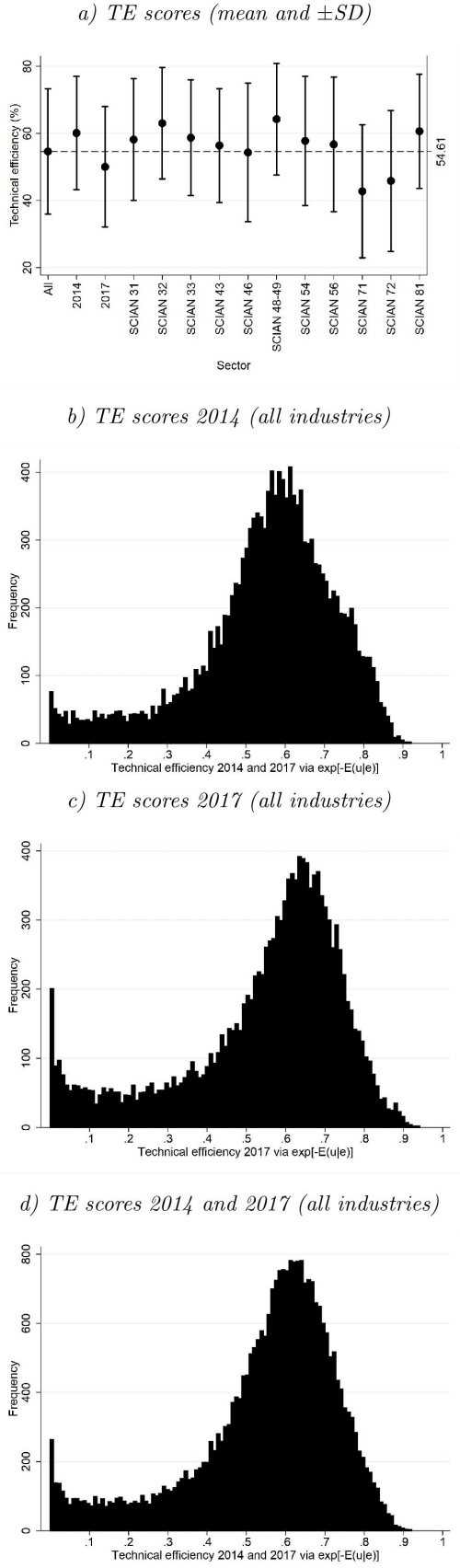
Source: Own elaboration based on parameter estimates in table 3.
Figure 1 Technical efficiency scores
4.2 Technical inefficiency
Table 4 shows the parameter estimates
Table 4 Parameter estimates of the technical inefficiency model
| Variables | All | 2014 | 2017 | SCIAN 31 | SCIAN 32 | SCIAN 33 | SCIAN 43 |
| Human | -0.0255*** | -0.0321*** | -0.0188*** | 0.0516 | -0.0453 | -0.0264** | -0.0078** |
| (0.0037) | (0.0066) | (0.0045) | (0.0757) | (0.0506) | (0.0131) | (0.0035) | |
| Patents | -0.2961 | -0.0887 | -0.9943* | -0.2014 | 2.5953 | -0.0061 | -0.4625 |
| (0.3153) | (0.4125) | (0.5169) | (3.4286) | (2.195) | (0.7473) | (0.4731) | |
| Licences | 0.0452 | 0.0435 | 0.0419 | -0.7067 | -0.4972 | -0.1063 | 0.0506 |
| (0.0514) | (0.0741) | (0.0752) | (0.8837) | (0.4981) | (0.1805) | (0.0614) | |
| Transfer | -0.7477*** | -0.7929*** | -0.7722*** | -4.5435* | -2.7826** | -0.3650* | -0.1454 |
| (0.0964) | (0.1584) | (0.1277) | (2.6285) | (1.1801) | (0.206) | (0.1085) | |
| Internet | -2.8016*** | -2.0905*** | -3.6798*** | -13.2739* | -7.2892** | -4.1016*** | -1.2211** |
| (0.3441) | (0.422) | (0.5379) | (7.687) | (2.8549) | (1.2364) | (0.4959) | |
| Taxob | 0.1132*** | 0.1084*** | 0.1229*** | 0.4189** | 0.2851*** | 0.1186*** | 0.0651*** |
| (0.0074) | (0.0112) | (0.0098) | (0.1931) | (0.0752) | (0.0193) | (0.0077) | |
| Export | 0.0134*** | 0.0146*** | 0.0137*** | 0.0366 | 0.0550** | 0.0222*** | 0.0048 |
| (0.003) | (0.0045) | (0.0041) | (0.0304) | (0.0224) | (0.0057) | (0.005) | |
| Managers | 0.0039 | -0.0037 | 0.0016 | -0.1172 | -0.1234 | -0.0478** | 0.0120** |
| (0.0056) | (0.0096) | (0.0071) | (0.1384) | (0.0772) | (0.0205) | (0.006) | |
| Sigma_U | 1.6000*** | 1.5071*** | 1.7341*** | 2.9265*** | 2.7635*** | 1.6100*** | 1.1018*** |
| (0.1) | (0.1598) | (0.1205) | (0.5728) | (0.334) | (0.2649) | (0.2121) | |
| Sigma_V | -0.8311*** | -0.6476*** | -1.1930*** | -1.2435*** | -1.2260*** | -1.2676*** | -0.5867*** |
| (0.0195) | (0.0249) | (0.0359) | (0.0934) | (0.0707) | (0.0765) | (0.0665) | |
| Observations | 28,034 | 14,557 | 13,477 | 2,269 | 2,278 | 2,913 | 3,563 |
| Log-likelihood | -37219 | -19650 | -16942 | -2497 | -2775 | -3483 | -5393 |
| SCIAN 46 | SCIAN 48-49 | SCIAN 54 | SCIAN 56 | SCIAN 71 | SCIAN 72 | SCIAN 81 | |
| Human | -0.0250*** | -0.0780** | -0.0196*** | -0.0160** | 0.011 | -0.02 | -0.0201 |
| (0.0062 | (0.0373) | (0.0075) | (0.0062) | (0.021) | (0.0128) | (0.0171) | |
| Patents | 1.1574*** | -3.4483 | -0.0954 | 0.1562 | -4.0069* | -1.0961 | -1.5353 |
| (0.4035) | (2.9073) | (1.068) | (0.4034) | (2.2264) | (0.9966) | (1.9103) | |
| Licences | 0.1728** | 0.486 | -0.0543 | 0.1126 | -0.796 | 0.1243 | 0.2986* |
| (0.0795) | (0.3411) | (0.1527) | (0.0692) | (0.6585) | (0.1656 | (0.1811) | |
| Transfer | -0.1125 | -1.3281* | -0.4206** | -0.0972 | -0.2208 | -1.1042** | -0.8158** |
| (0.117) | (0.7156) | (0.2001) | (0.1279) | (0.5994) | (0.487) | (0.3664) | |
| Internet | -2.9148*** | -4.1019*** | -4.0685*** | 0.5416 | -1.6479 | -0.636 | -1.9013* |
| (0.5487) | (1.5808) | (1.5514) | (0.4985) | (1.7583) | (0.4597) | (1.137) | |
| Taxob | 0.0809*** | 0.1539*** | 0.1206*** | 0.0445*** | 0.0961** | 0.0997*** | 0.0852*** |
| (0.0086) | (0.0429) | (0.0235) | (0.0096) | (0.041) | (0.0263) | (0.0199) | |
| Export | 0.0230*** | -0.001 | 0.0208* | -0.0015 | -2.3763* | -0.0841 | 0.0343*** |
| (0.007) | (0.0126) | (0.0118) | (0.0057) | (1.4078) | (0.1565) | (0.0087) | |
| Managers | 0.0102 | 0.0235 | -0.0049 | -0.0025 | -0.0253 | -0.0234 | 0.0353* |
| (0.007) | (0.0147) | (0.0167) | (0.006) | (0.0341) | (0.0197) | (0.0196) | |
| Sigma_U | 1.3419*** | 1.6422*** | 1.4389*** | -0.5075 | 1.3475** | 1.1502*** | 1.0107** |
| (0.1707) | (0.4681) | (0.2854) | (0.7987) | (0.5513) | (0.3968) | (0.4501) | |
| Sigma_V | -0.8998*** | -0.8633*** | -0.7747*** | -0.4876*** | -0.7809*** | -1.0233*** | -0.7529*** |
| (0.0455) | (0.0602) | (0.0433) | (0.1124) | (0.1493) | (0.0643) | (0.0874) | |
| Observations | 4,767 | 2,568 | 3,274 | 1,170 | 327 | 3,704 | 1,201 |
| Log-likelihood | -6798 | -3193 | -4144 | -1576 | -418.9 | -4248 | -1541 |
Notes: Dependent variable: Technical inefficiency. Robust standard errors in parentheses. *** p<0.01, ** p<0.05, * p<0.1.
Source: Own elaboration based on INEGI (2015, 2018).
In most industries, applications to register patents are not statistically significant, which indicates that the creation of knowledge has no effect on TE scores of SMEs in Mexico. According to Holgersson (2013), who conduct a literature review on patent management in SMEs, the main constraint for patenting in SMEs is their lack of resources in the application stage and for monitoring and enforcing their patents. The no significance of these terms may indicate that liquidity constraints prevent SMEs from making large investments in creating new technologies. In this regard, Lanjouw and Schankerman (2004) and Kingston (2004) argue that the patent system does not work properly for SMEs because such enterprises are more exposed to litigation risks and threats than large firms, which can deal with such litigations and threats more easily. Given such obstacles, SMEs may be adapting existing technologies to their productions processes rather than allocating their production efforts to create new knowledge.
According to table 4, we do not find empirical evidence that validates the previous hypothesis. It seems that the acquisition of existing technologies does not influence TI scores. Buying licences and adapting existing technologies to the production process without any modification (more frequently) does not lead to higher efficiency. The cases in which such a hypothesis holds are the retail trade sector and other services. Regarding transfers of knowledge to another enterprise, SMEs that create and sell new technologies to another enterprise more often tend to be less efficient than other SMEs. This finding is not in line with our original expectations; however, it might be explained by the creation of comparative advantages of those firms creating new technologies but not selling them to other firms. Furthermore, since SMEs do not generally create new forms of knowledge, transfers to other enterprises might not take place frequently. Using the Internet in the production activities strongly improves SMEs performance in most industries, especially in the manufacturing, transport, mail and storage, and professional, scientific and technical services sectors, where Internet connection is used intensively.
Our results add further support to the argument that expenses related to the tax payment procedures push SMEs away from the frontier. This association is strongly significant in all industries and both years. For policymakers, such a finding represents an opportunity because simplifying the required procedures for paying taxes would likely benefit TE of SMEs and, at the same time, boosts the economic recovery. Managerial practices are also hypothesised to influence firms’ performance. In this paper, we discover that the number of managers per worker generally has no effect on TI. As exceptions, in the 33 manufacturing industries (wholesale trade and other services) increasing (reducing) the number of managers would likely reduce (increase) TI. Perhaps, the existence of non-monotonic effects explains such results. That is, there exists a turning point at which the number of managers per worker is optimal and the slope of this relationship is reversed. This is something that should be analysed using the non-monotonic effects suggested by Wang (2002).
Using parameter estimates in table 4 and equation (6), we compute firm-specific marginal effects of each control variable on TI. Figure 2 shows the average and ± 1.96 SD marginal effects for the 8 explanatory variables and for different samples. In line with parameter estimates in table 4, higher proportions of employees with a bachelor’s degree tend to reduce TI. On average, a 10% increase in such a proportion leads to a 3% reduction in TI. The only exceptions are the 31 and 71 NAICS industries, where most of the firm-specific marginal effects are close to zero (see figure 2a). Although SMEs that asked for a patent are on average 2.9% more efficient than other SMEs, most of the firm-specific marginal effects in different industries are close to zero. There are some exceptions. SMEs in the 43, 71, 72, and 81 NAICS industries that applied for a patent are on average 11.3%, 38.7%, 9.1%, and 18.7% more efficient than other SMEs in the corresponding industries (see figure 2b).
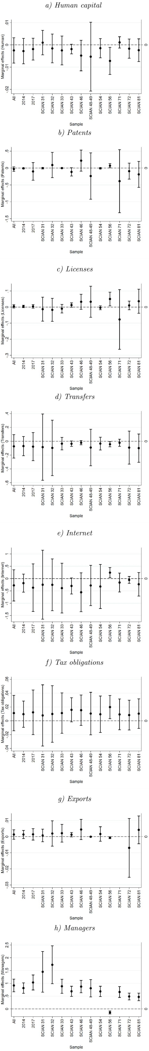
Note: We exclude the 71 NAICS industry in the 2g figure due to scale issues. The average marginal effect in the 71 NAICS industry is -0.23. Source: Own elaboration based on Wang (2002) and INEGI (2015, 2018).
Figure 2 Distribution of firm-specific marginal effects
We also observe heterogeneity of firm-specific marginal effects of licenses and transfers among industries. Regarding licences that allow SMEs to use existing technologies in their production processes, most of the marginal effects are close to zero. However, SMEs in the 46, 48-49, 56, and 81 NAICS industries that rarely buy these licences tend to be more inefficient than their counterparts. On average, reducing the frequency of technology acquisition by one unit increases TI scores by approximately 0.45% in the pooled sample (see figure 2c). In terms of transfers, we observe that SMEs selling their own technology to other firms less frequently are, on average, more efficient than those SMEs doing it regularly. Our results indicate that reducing the frequency of technology transfers by one unit shrinks TI scores by approximately 7.4% in the pooled sample (see figure 2d). Furthermore, if the firm uses the Internet in its production processes, it is, on average, 27.6% more efficient than those without access to the Internet (see figure 2e).
We confirm that costs related to tax payments generally boost TI. On average, a 1% increase in the ratio of such costs to total revenue rises 1.12% TI scores in the pooled sample. In all other samples, we observe that the average marginal effect is above the zero line, which suggests that the complexity of tax payments’ procedures may create technical inefficiencies in the production process thereby such financial resources should be used in a more efficient way (see figure 2f). Our findings for marginal effects of the share of exports on TI contradict the initial expectations in most industries. A 1% increase in exports share leads to 0.13% rise in TI scores in the pooled sample. The exceptions are the 48-49, 56, and 72 NAICS industries, for which the average marginal effects are -0.01%, -0.07%, and -22.97%, respectively. This finding deserves further exploration, especially in large firms that are more likely to be linked to the external market (see figure 2g). Finally, we find that the current ratio between managers and the total number of employees in SMEs may be beyond the optimal level, implying that additional managers would likely increase TI scores (see figure 2h).
4.3 Discussion
The results indicate that SMEs in the manufacturing, trade, and service sectors are not fully efficient. This implies that such enterprises can either produce more output using the same inputs more efficiently or produce the same output using fewer inputs. We also encounter that human capital, measured by the share of employees with a bachelor’s degree to total workers and the use of the Internet in the production activities, reduce TIs. On the other hand, when SMEs spend large quantities of money on tax payments procedures, such firms tend to be less efficient than their counterparts. The results are not conclusive and sector-specific for the remaining inefficiency effects.
To contextualise our findings, we compare them with previous research in table 1. Figure 3 shows ATEs reported by studies where Mexico is the case of interest. The first 10 studies use the DEA and the rest the SFA models. Overall, we observe lower ATEs in SFA than in DEA studies, but our results coincide with those using the same approach. The comparisons among studies are not always possible because the corresponding samples and industries of interest are not the same. However, our results for ATEs are in line with those in Aguilar (2011), Chavez and Fonseca (2012), Valderrama et al. (2015) and Diaz et al. (2019), who analyse manufacturing and automotive industries.
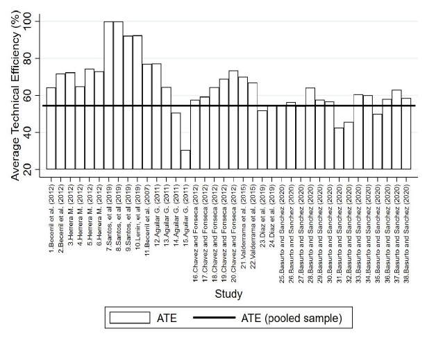
Notes: 1. All (CRS); 2. All (VRS); 3. Manufacturing (micro); 4. Manufacturing (small); 5. Manufacturing (medium); 6. Manufacturing (large); 7. Automotive (2004); 8. Automotive (2009); 9. Automotive (2014); 10. Electric (BC); 11. All; 12. Manufacturing (footwear); 13. Manufacturing (garment); 14. Manufacturing (wood); 15. Manufacturing (textile); 16. Manufacturing (1988); 17. Manufacturing (1993); 18. Manufacturing (1988); 19. Manufacturing (2003); 20. Manufacturing (2008); 21. Manufacturing (1985); 22. Manufacturing (2009); 23. Automotive (1988); 24. Automotive (2008); 25. All (11 NAICS); 26. All (11 NAICS-2014); 27. All (11 NAICS-2017); 28. Manufacturing (31 NAICS); 29. Manufacturing (32 NAICS); 30. Manufacturing (33 NAICS); 31. Wholesale trade (43 NAICS); 32. Retail trade (46 ; NAICS); 33. Transport, mail and storage (48-49 NAICS); 34. Professional, scientific and technical services (54 NAICS); 35. Business support, waste management, and remediation services (56 NAICS); 36. Cultural and sports entertainment and other recreational services (71 NAICS); 37. Temporary accommodation and food and beverage preparation services (72 NAICS); 38. Other services except government activities (81 NAICS). Source: Table 1 and figure 1a.
Figure 3 Average Technical Efficiency: A comparison
Some of the results are in line with the existing empirical literature. For example, Taymaz (2005), Aguilar (2011), Charoenrat et al. (2013), Valderrama et al. (2015), and Diaz et al. (2019) also discover that better endowments of human capital significantly reduce TIs, which adds further empirical support to the argument that high-qualified workers help to use available resources more efficiently. Regarding the use of the Internet, or ICTs, Becchetti et al. (2003) also find that its use reduces TI in Italian manufacturing firms, arguing that such tools positively affect the creation of new processes or products. We also argue that the Internet facilitates the flow of knowledge and market information towards and out of SMEs. The positive association between the expenses incurred by the firm for tax payments and TI is in line with our initial expectations. There are many studies in the literature looking at the subsidies or taxes- TI link; however, this information is not available in ENAPROCE. Therefore, we could not account for it in the TI equation. Assuming that such expenses are highly correlated with tax payments, our results suggest that, on average, current taxes significantly increase TI in SMEs. On the other hand, if such costs are not correlated with tax payments, policymakers should simplify tax payments procedures to reduce TI in SMEs.
Taymaz and Saatci (1997) find that technology transfers significantly reduce TI. However, Becchetti et al. (2003) and Taymaz (2005) encounter that such a relationship is not statistically different from zero. Our results are in line with the latter findings, i.e., the way in which they use available inputs remain unchanged. Regarding knowledge creation, we find that requests for registering patents are not associated with TI. However, SMEs creating and selling their own technology to other firms less frequently are, on average, more efficient than those doing it more frequently. This result suggests that SMEs prefer not to sell their innovations and create comparative advantages instead.
Bigsten et al. (2000) and Tovar (2012) find that firms selling their output in the external market are, on average, more efficient than other firms; notwithstanding, Alvarez and Crespi (2003) encounter a null association, and Diaz et al. (2019) the opposite relationship. Our findings align with Diaz et al. (2019) and Alvarez and Crespi (2003). However, given our data’s cross-sectional nature, we think that omitted variables might cause a bias in the parameter estimates and can be explored carefully in future studies. For the share of managers over total employees, the results are in line with Taymaz (2005), who do not find a statistically significant association between administrative personnel and TI. We argue that such a relationship should be analysed at the firm level and see whether the current level of managers per worker is optimal or not.
Unfortunately, we could not account for all inefficiency effects in the TI equation. Among other things, the existing literature suggests the inclusion of investment in R&D activities, training for employees, debts, firm experience (years in the market), specialization indexes, etc. (see table 1). Although some of these variables appear in the ENAPROCE, there are many records with missing information, preventing us from including them as inefficiency effects in the TI equation. Therefore, the reader should consider this limitation, and we encourage future studies to analyse such effects once the data becomes available.
5. Conclusions
This paper investigates the knowledge- TE association using data on 28 034 SMEs from Mexico’s manufacturing, trade and services industries. We use the single-step SFA to compute firm-specific TE scores. The main findings indicate that the ATE in the sample is 54.6%; that is, SMEs can produce more using the current inputs more efficiently or produce the current output using fewer inputs. We hypothesise that different types of knowledge, human capital, innovation, and technology transfers from and to the firm determine the gap between the observed and the maximum attainable output, TI. Our results indicate that human capital, creating and selling new technologies to other firms less frequently and using the Internet in production activities significantly reduce TI. On the other hand, firms are, on average, less efficient when they spend large amounts of money on the required tax payments procedures. The results for the remaining inefficiency effects, patent applications, exports, licences to use existing technology, and managers per employee are not conclusive.
We contribute to the existing literature as follows. First, this study provides empirical evidence on how different types of knowledge relate to TE in SMEs, which typically face liquidity constraints that prevent them from investing in creating new knowledge. The analysis of the knowledge- TE link allows us to test whether putting efforts on the creation/acquisition of knowledge can help SMEs to use inputs more efficiently or not. If so, policymakers should use this channel to reduce production inefficiencies in the economy. Second, this research provides policymakers with useful information about SMEs’ performance and inefficiency effects that can be used to support policies aiming to attenuate the harmful effects of the 2020 global recession. Under the current global economic context and following the main results of this research, SMEs would likely use fewer inputs to produce the same output, even less, than before the pandemic. For the economic recovery, SMEs should use their available inputs more efficiently, and that can do it by investing in human capital and innovations that improve their production processes. This is particularly relevant because SMEs hire approximately 3.2 million employees in Mexico.
In line with our initial expectations, SMEs spending larger amounts of money on tax payments procedures are less efficient than their counterparts. Under such circumstances, policymakers should simplify tax payments procedures to reduce harmful effects on TE of SMEs, especially in the economic recovery. Notice that we do not analyse tax payments as inefficiency effects in the TI equation. As in other studies, such as Diaz et al. (2019) and Alvarez and Crespi (2003), we do not find solid evidence that firms exposed to the external market are more efficient than those participating in the domestic market.
The reader should be aware of some caveats of this research. First, data availability prevents us from carrying out the analysis for large and micro-sized firms in Mexico and from including all inefficiency effects suggested by the existing literature. Second, although ENAPROCE reports data from 2014 and 2017 and some firms appear in both surveys, the time frame is still not enough to identify structural changes over time. Further steps of this research should: i) include tax payments in the TI equation to test whether such payments enlarge TI or not; and ii) carry out the analysis using data on large firms to test whether the knowledge- TE association is stronger than in SMEs or not, because large firms more likely invest in the creation of knowledge.

