nueva página del texto (beta)
 Inglés (pdf)
 Artículo en XML
 Referencias del artículo
 Enviar artículo por email
 Citado por SciELO
  Similares en
SciELO
Similares en
SciELO 
 Permalink
1. Introduction
The reading of the economic cycle is essential to the formulation and implementation of monetary policy. Economic indicators such as the gross domestic product, credit indicators, interest rates, and unemployment can help to assess the current stage of the business cycle and thus the appropriate policy stance. The analysis is even more sensitive when there is a transition from an expansionary stage of the economy to a contractionary one, or vice versa. An important topic in monetary policy focuses on whether employment is approaching its potential: the rate of unemployment at which inflation remains constant in the absence of supply shocks. This rate is called the non-accelerating inflation rate of unemployment (NAIRU). However, the estimation of the NAIRU is complicated, because it is not directly observable. In Mexico and other Latin American countries, the presence of a sizeable number of informal workers imposes an additional challenge. The existence of unions, the degree of centralization in the bargaining process, distortions caused by labor legislation, the existence of monopolies, and other factors could limit labor market flexibility in the formal sector. However, the lack of labor regulation in the informal sector official promotes a competitive equilibrium and greater wage adjustment in that market.
Given that Mexico does not have unemployment insurance, workers who become unemployed immediately face the pressure to find a new job. The wage flexibility of the informal sector allows it to absorb most of the people who cannot find a job in the formal labor market; and workers who would otherwise be unemployed can find a job there. As a result, the unemployment rate in Mexico is low: it includes only frictional unemployment and a fraction of the cyclical unemployment that is absorbed by the informal sector.
Given these particular characteristics of the Mexican labor market, it is possible that the unemployment rate does not fully reflect the labor market slack. We thus estimate measures of labor market slack, first using the traditional unemployment rate, and then complementing this analysis with a new indicator of labor market underutilization that includes a measure of informality by including both unemployed workers and informal wage earners. Using standard methodologies, we estimate the NAIRU over time using both the traditional unemployment rate (NAIRU-trad) and the modified unemployment rate that takes informality into account (NAIRU-inf).
It is important to allow the NAIRU to vary over time because changes in this rate could be related to changes in structural labor market conditions such as flexibility, competitiveness, productivity, and demographic changes that alter the composition of the economically active population, as well as other institutional or policy issues.1 In general terms, the NAIRU may present variations due to structural changes in the fundamental factors affecting labor supply and demand.
We find that the NAIRU and labor market slack follow similar patterns over time using either indicator of labor market underutilization. However, according to an endogenous threshold model, the indicator including informal wage earners seems to predict inflationary pressures better when the unemployment gap is close to zero; as a result, it appears to anticipate the inflationary pressures observed in 2007-2008 more clearly than the traditional slack indicator. In addition, both estimates show labor market slack decreasing throughout 2016 and approaching zero. The indicator taking informality into account shows relatively more slack, which is consistent with the absence of significant wage pressures observed during this period. Given these results, we conclude that it is important to assess the level of labor market slack in the economy using measures like the NAIRU as estimated in this paper, and that analysis of the economic cycle can be effectively complemented by considering informal employment. This method could be a convenient tool for monetary policy, particularly in countries like Mexico and other emerging economies with significant informal labor.
The rest of this paper is organized as follows: in section 2, we explain how informal employment relates to labor market slack. In section 3, we present the data sources and the methodology to estimate both measures of the NAIRU. Section 4 describes our results. Section 5 provides additional information about the Mexican labor market throughout the economic cycle, and section 6 offers some conclusions.
2. Informal employment and labor market slack
One of the key features behind the presence of informality in some economies is the low flexibility of their labor markets. Different degrees of flexibility in formal and informal labor have implications for the cyclical adjustment of labor markets. During recessions, for example, wage flexibility in the informal sector allows the market to absorb individuals who do not find formal employment: workers who would otherwise be unemployed. This dynamic would imply that the informality rate is countercyclical a stylized fact amply documented in the literature (see, for example, Chiquiar and Ramos Francia, 1999; Alcaraz, 2009; Gasparini and Tornarolli, 2009; Fiess et al., 2010; Perry et al., 2007; and Peterson, 2014).2 Figure 1 shows the evolution of the informality rate and the output gap in Mexico, which indeed suggests that the informality rate in the Mexican economy follows a countercyclical trajectory.3
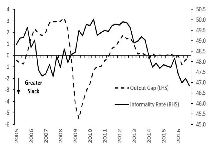
Note: The output gap is shown as a percentage of potential GDP. We calculate informality in urban areas with a population larger than 15,000.
Source: Authors’ calculations using data from ENOE and INEGI.
Figure 1 Informality rate and output gap %
With these considerations in mind and given the characteristics of the Mexican labor market, Mexico’s unemployment rate is low, as it tends to include only part of cyclical unemployment. Chiquiar and Ramos Francia (1999) were the first to note that for this reason, the unemployment rate in Mexico may not adequately reflect labor slack. However, they did not use informal labor to measure labor market slack or estimate a NAIRU that includes informal labor. To our knowledge, the present study is the first in which data for informal labor has been used to obtain additional information about the economic cycle and labor market slack.
The lack of regulation of the informal sector is the most obvious explanation of its flexibility. In Mexico, the Federal Labor Law (Ley Federal del Trabajo, LFT) aims to promote safe working conditions for wage earners by defining minimum wages and benefits and regulating union activity and labor contracts. For instance, Article 23 requires that those who have worked for an employer for more than a year are entitled to a severance payment equal to three months’ wages if laid off or fired. The complete absence of labor regulation in the informal sector simplifies the hiring and firing of workers. There is no need to comply with the costly bureaucratic requirements typically found in the formal sector, such as enrolling workers in social security and registering them with the tax authorities. The absence of union activity in the informal sector is also an important determinant of its flexibility. The process of hiring a worker is usually even more difficult if a firm has a unionized workforce because unions impose substantial restrictions on hiring and firing workers, and act as a strong source of pressure in the negotiation of wages.
There are ways to explain the differences in wage flexibility between the formal and informal labor markets which do not assume that regulations affect each sector differently. Esfahani and SalehiIsfahani (1989 link effort observability with informality in a theoretical model, using efficiency wage theory; they argue that the main characteristics of the informal sector (small firm size, low-skill workers, and low technological level) are associated with higher levels of effort observability and more competitive wages, which imply greater flexibility and no involuntary unemployment. In the formal sector, however, with lower levels of effort observability, wages are usually above the reservation wage level, which promotes lesser flexibility and involuntary unemployment. More recent studies have proposed integrated labor markets with frequent transitions between informal and formal jobs. For example, Maloney (1999 argues that in Mexico there is no segmentation, and that informality exists because some workers want to take advantage of the dynamic and unregulated informal labor market. Meghir et al. (2015 propose an equilibrium wage-posting model with heterogeneous firms that decide to locate in the formal or informal sector and workers who search randomly on and off the job. However, some authors have also argued the possibility of a heterogeneous labor market where part of the informal sector is voluntary, while the other includes workers who would like to obtain a formal job but cannot get it because of the barriers created by regulation (see, for example, Perry et al., 2007). Therefore, even if part of informal labor is voluntary and integrated with the rest of the economy, we might still observe a countercyclical informality rate.
2.1. Labor and economic activity indicators of slack
A standard national accounts statistical procedure is to update the base year to estimate the Gross Domestic Product (GDP) series. This process includes an important effort by the Mexican National Institute of Statistics and Geography (Instituto Nacional de Estadística y Geografía, INEGI) to update the value of the different goods produced in the economy. The GDP series is thus more accurate and the historic GDP series changes, both in terms of level and growth rates. This change may affect the measurement of economic activity and, as a result, the estimation of economic activity slack in real-time.4 However, labor market slack is not subject to this problem, because the variables used to compute this indicator are generally based on the number of employed or unemployed workers and is not subject to periodic revisions. These considerations highlight the importance of taking labor market information into account to evaluate slack in the economy in real-time.
2.2. Informal labor definition and identification
According to international criteria proposed by the International Labour Organization (ILO, 2003), informal workers include self-employed persons and wage earners not registered in social security. Some informal workers, particularly the unregistered self-employed, may earn relatively high incomes and may work voluntarily in the informal sector, that is, they remain informal even if they have an opportunity to enter the formal sector. In contrast, involuntary informal workers-those who would rather have formal employment but cannot obtain ittend to concentrate in the group of informal wage earners (see Alcaraz et al., 2015; and Fajnzylber and Maloney, 2007). The World Bank flagship report Informality Exit and Exclusion (Perry et al., 2007) finds that informal wage workers are more disadvantaged than their informal self-employed counterparts in several Latin American countries. Alcaraz et al. (2015) use a model of self-selection with entry barriers into the formal sector to detect endogenously involuntary informal workers and find a higher proportion of involuntary informal workers among wage workers. Informal wage earners may thus best represent disadvantaged workers and, consequently, behave similarly to unemployed workers. We therefore combine informal wage earners and unemployed workers to construct our extended indicator of slack in the Mexican labor market, defined as the extended indicator of the level of unemployment consistent with an environment of stable inflation. We use this indicator to analyze the evolution of slack in the Mexican labor market from 2005 to 2016. To evaluate the advantages of using this variable as an alternative to traditional measures, we also estimate the NAIRU using only the unemployment rate (NAIRU-trad) and compare the slack estimated with both indicators (slack-inf and slack-trad). By comparing these indicators through different stages of the economic cycle, we can evaluate their ability to indicate inflationary pressures.
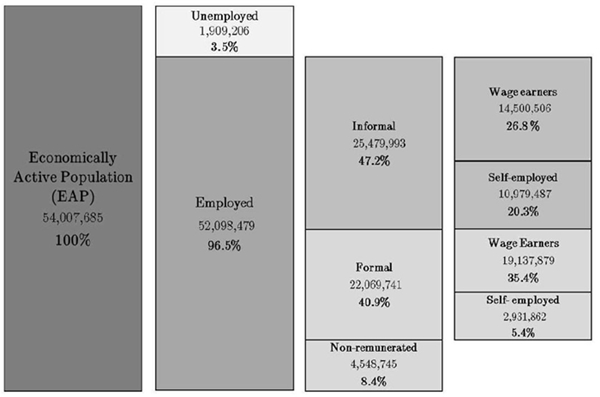
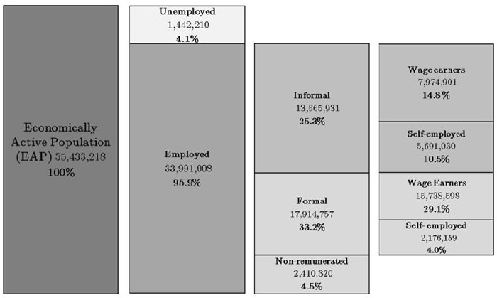
In order to assess the participation of our proposed new indicator of labor slack slack-inf within the Economically Active Population (EAP), we calculate the EAP composition from the National Survey of Occupation and Employment (Encuesta Nacional de Ocupación y Empleo, ENOE) data, using expansion factors to obtain population-representative data, as shown in figure 2.5 The data correspond to the survey of the fourth quarter of 2016. Among the population aged 15 years and older, just over 35 million are economically active, and of these, 4.1 percent were unemployed. There were just under 34 million who were employed, almost 13.7 million of them were informal. In turn, informal wage earners (informal employees) represented 14.8 percent of the EAP in the fourth quarter of 2016. Our alternative rate of unemployment, taking informal labor into account, was 26.6 percent (the traditional unemployment rate of 4.1 percent plus the informal wage earners’ rate of 22.5 percent). It is important to notice that non-remunerated workers (workers that receive no wage) represented 6.8 percent of the EAP. These workers earn some kind of non-monetary income but it is not observable. Furthermore, in general, these workers have a particular type of labor relationship associated with family activity. In line with other empirical labor market studies, we exclude these workers from our analysis.
2.3. Exogenous policy changes that could trigger changes in incentives between formal and informal labor
One potential problem with our alternative measure of slack is the possibility of legal or administrative actions aimed at reducing informal employment in the economy. If these measures are successful, such a reduction could take place regardless of the economic cycle, resulting in an erroneous attribution of the decline to the slack in the economy. We argue that this problem is not severe enough to offset the usefulness of our alternative indicator. Unfortunately, we can only provide circumstantial evidence for some cases, but for the rest, we have administrative data that allows us to quantify the effect of these measures on the number of formal workers.
Since our empirical strategy allows for changes in the NAIRU over time, we do not expect that gradual changes in the informality rate caused by these measures will bias our results. In order to assess the magnitude of this problem, we list in table 1 all the actions taken during the study period that encouraged worker registration, and we link them to the informality rate over time (see figure 1). Mexico’s primary social security institution, the Mexican Social Security Institute (Instituto Mexicano del Seguro Social, IMSS), regularly sponsors campaigns to encourage formalization of employment. However, none of these campaigns seem to have resulted in a significant decrease in informal employment. The government also promoted a series of ‘first job’ programs encouraging young workers to register in 2007 and 2010. According to administrative data, these programs registered 25,000 workers per year. If we consider that approximately 700,000 new workers register at IMSS every year, it is clear that these programs did not meaningfully increase formality during the time span of our analysis.
Table 1 Policy measures possibly affecting informal employment in Mexico, 2000-2014
| Period | Policy/Program |
Effects on formal employment |
2000-2014 |
IMSS implemented various measures to increase formal employment registration. |
No information available. |
2007 |
First Job Program (Programa de Primer Empleo) |
From 2007 to 2011, these programs increased the number of young formal workers by approximately 25,000 per year, on average. |
2010, relaunched in 2011 |
First Job Promotion Program (Programa de Fomento al Primer Empleo) |
|
2012 |
Federal Labor Law reform |
Banco de México (2012) predicts a gradual increase in informality, mainly among young and part-time workers, including women, students, and the elderly. |
2013 |
Employment Formalization Program |
No information available. |
2014 |
Agreement between IMSS and the tax authorities to share information about registered workers. |
This measure may have had an impact on the formalization of employees. |
2014 |
‘Crezcamos Juntos’ Program |
The number of new formal workers registered in the tax system has increased since the start of the program, but there has been an insignificant increase in the number of workers registered for social security (IMSS). |
Source: IMSS, Federal Labor Law, Secretaría del Trabajo y Previsión Social, Servicio de Administración Tributaria.
In 2012, the Mexican Congress approved a labor law reform, which may have encouraged the registration of wage earners (see Banco de México, 2012). However, according to the Banco de México, the increase in the number of formal workers due to this reform would be gradual, over a few years. Given that our methodology allows for changes over time in the NAIRU, we do not consider this reform as a serious source of bias in our analysis. In 2014, the government launched the program Crezcamos Juntos (‘Let’s Grow Together’) to encourage the registration of small firms. This program might have led to an increase in the number of registered workers and thus a reduction in informal employment, but the increase was negligible. Finally, in the same year, IMSS and the tax authorities agreed to share information about registered workers. It is advantageous for employers to register workers and wages with the tax authorities because they receive tax deductions, but there is also an incentive not to register workers with IMSS, as the employer pays part of the cost of social security. It was expected that as a result of the sharing agreement, employers with more workers registered with the tax authorities than with IMSS would increase IMSS registration, so the numbers would match. This measure could thus have induced the formalization of workers. However, the effect of this measure might be limited by the fact that employers may assume that both institutions shared information with no need of agreement, and as a consequence, they regularly matched the workers’ registration in both institutions independently of the celebration of any agreement.
Figure 1 shows an important variation of informality over time, but we observe no relationship with any of the policy measures explained in this section. Even though there have been some changes in regulations that could bias our results, we conclude that the magnitude of this problem is not significant enough to affect them.
3. Modeling inflation dynamics and the NAIRU in Mexico
3.1 Econometric methodology
There are different methodological approaches in the literature to estimate the NAIRU and thus to calculate the corresponding unemployment gap. In this paper, we focus on the estimation of the NAIRU from equations that model inflation dynamics based on the Phillips curve. The consensus in the literature is that the most suitable conceptual framework for studying the NAIRU is a reduced-form Phillips curve approach. We use this approach to compute the NAIRU as the unemployment rate consistent with stable inflation, subject to an expectations-augmented Phillips curve. This relationship broadly establishes a negative link between inflation and the unemployment gap the difference between the observed unemployment rate and the NAIRU in the short run, such as the following:
where:
In order to better approximate the dynamics of the inflationary process, we generalize this relationship and, following Staiger et al. (1997a and 1997b), we use the following empirical model to estimate inflation dynamics:
where:
The literature on the estimation of the NAIRU includes different interpretations of these ways of modeling inflation. Gordon (1997 deliberately omitted inflation expectations and estimated the NAIRU from what he calls the triangle model of inflation. According to this model, the inflation rate depends on three basic determinants: inertia, demand, and supply. Staiger et al. (1997a) develop another interpretation: the random-walk model for inflation expectations, i.e.,
Our methodological strategy is first to estimate a version of equation (1) for each of our two measures of unemployment in Mexico, assuming the NAIRU is constant. From this estimation, we conduct a simple statistical test with the null hypothesis of constant parameters (Chow test) that suggests that the NAIRU in Mexico might have changed in recent years. From these first results, we estimate models that allow us to obtain a time-varying NAIRU. Specifically, we consider two reduced-form approaches widely used in the literature: i) a deterministic NAIRU, i.e., a recursive estimation from equation (1), and ii) state-space specifications, which provide further flexibility regarding the dynamic properties of the NAIRU. We explain these specifications in further detail below.
NAIRU recursive estimation
In the specification of equation (1), the unemployment gap could have a contemporaneous and a lagged impact on inflation. In order to simplify the NAIRU estimation, we assume that
such that if
However, in order to allow the relationship between unemployment and inflation to vary over time, we compute the path of the NAIRU through a recursive estimation of equation (2), leaving the starting point of the sample fixed as follows:
Through this estimation, it is possible to infer the evolution of the NAIRU over time, since the most recent information is incorporated into the model. An alternative strategy could be a rolling window estimation of the model, but the size of the sample and the drastic behavior of the unemployment rate in the international financial crisis make these estimates very volatile.8
We model the NAIRU as an unobserved stochastic process, where we assume that its determinants are unknown but persistent (i.e., they follow a random walk). Starting from the simplest case, components that further explain the dynamics of the unemployment rate, such as lags and the output gap, can be gradually added to the system of equations to introduce additional structure into the model. We describe below the three cases we explore.9
NAIRU random walk
As in Gordon (1997, the evolution of the NAIRU is obtained from the following system of equations:
where errors are assumed to be i.i.d. N
NAIRU random walk and AR(2) unemployment gap
In addition to assuming a random-walk NAIRU, this methodology models the dynamics of the unemployment gap
Where
NAIRU random walk and unemployment gap (Okun’s Law)
We expand the previous system of equations with the inclusion of an equation relating the unemployment gap to the output gap (Okun’s Law). The system of equations we use to estimate the NAIRU is the following:
Where
3.2 Data
We use monthly, seasonally-adjusted data for unemployment and prices from January 2005 to December 2016, obtained from INEGI. In all estimations, inflation
The data on informal wage earners comes from INEGI’s ENOE, a quarterly household survey with a rotating panel structure, from 2005 to 2016. Every quarter, INEGI replaces one-fifth of the sample: each household is thus followed for five consecutive quarters. The purpose of the survey is to collect data on the employment situation of Mexicans aged 15 and older in rural and urban areas. It is possible to identify informal wage earners in this survey, as defined by the ILO (2003). We assume that workers are informal if they are wage earners without any of the following mandatory benefits: IMSS (social security), ISSSTE (social security for government employees), Afore (retirement benefits), INFONAVIT (home loan), or private health insurance. For comparability purposes, we convert the quarterly informal labor data to monthly data using linear interpolation15 because the rest of the variables considered are available as monthly data.16
In the baseline estimation, unemployment
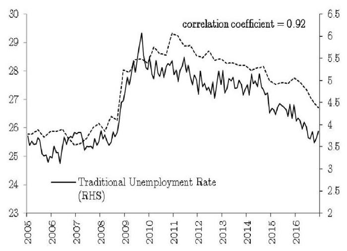
Source: INEGI and authors’ calculations with data from ENOE, INEGI
Figure 3 Traditional and extended unemployment rate %
We estimate the output gap
4. Estimates of the NAIRU
4.1 Results A first approach to the NAIRU
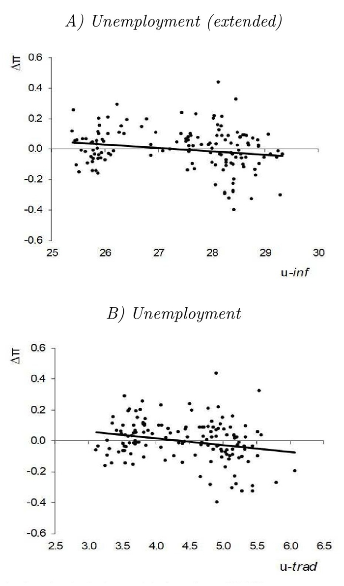
Figure 4 shows scatter plots of the change in annual inflation against the two measures of unemployment. First, it should be noted that there is indeed a negative relationship between the variables. The correlation between the changes in annual inflation and
Source: Authors’ calculations with data from INEGI.
Figure 4 Relationship between the change in annual inflation and unemployment in Mexico, 2005:01-2016:12
From the intersection of the line of best fit with the x-axis (i.e., when the change in inflation is zero), we can infer that the NAIRU-trad is 4.4 and the NAIRU-inf is 27.3.18 However, this analysis would omit the inertial effects of inflation and the possible effect of supply shocks. The results of the estimation of equation (1) for both measures of unemployment are shown below.19
NAIRU-inf:
NAIRU-trad:
Where
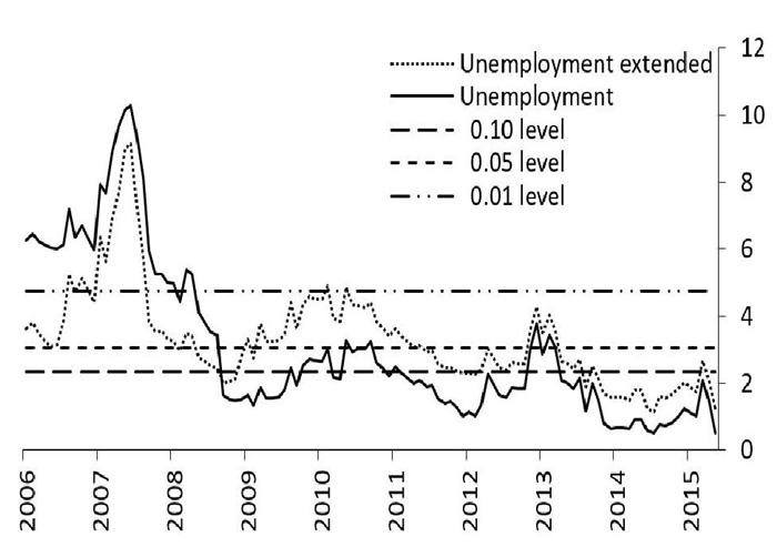
From these results, we observe that both the traditional unemployment measure and the proposed indicator have statistically significant effects on inflation. We also obtain a first estimate of the NAIRU, where we assume it is constant over time. Under this assumption we obtain NAIRU-trad = 4.43 (0.27) and NAIRU-inf = 27.46 (0.48).22 We test the assumption of a constant NAIRU by applying a test of structural change, the classical Chow test of structural change with the null hypothesis of constant parameters,23 which divides the sample in two and tests whether the coefficients related to the NAIRU estimation are equal in both subsamples. Figure 5 illustrates the results of this test for different periods. In most periods the null hypothesis of constant parameters is rejected at the conventional significance levels. We can thus conclude from the analysis that the NAIRU-trad and the NAIRU-inf show trajectories that vary over time.
Time-varying NAIRU
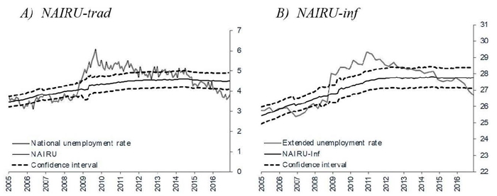
We next present in graphical form the results of the methodologies for estimating a time-varying NAIRU for both measures of unemployment. Appendix B presents detailed results for each estimated model. In figure 6, we show the results of the NAIRU and labor market slack using both the traditional indicator of labor underutilization, unemployment (slack-trad), and the extended indicator (slack-inf), estimated with the four models described in the previous section. In general, our results show that the estimations of both NAIRU-trad and NAIRUinf increase slightly over time, and that slack-trad and slack-inf follow a similar trajectory.
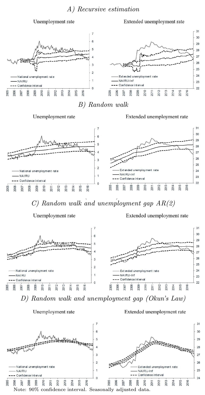
Now we compare the four estimations, highlighting their major differences. The recursive estimation seems to jump slightly in mid2009 and then start a slight upward trend through the end of the sample period. These jumps are not observed in any of the state-space models because those are estimated with double smoothing using the Kalman filter. However, we can see that all the specifications coincide in a final NAIRU that is greater than at the beginning of the period. If we focus on the three state-space models, which differ only in how we model non-observable variables, we can distinguish some of the modeling differences. For example, the results of the random-walk model show a NAIRU with a clear upward trend, which slows down in the final years of the sample. These results contrast with those of the model in which the unemployment gap follows a second-order autoregressive process (see equation 4). In this specification, the unemployment gap tends to revert to its zero mean, which makes the slope of the NAIRU flatter than that of the random-walk models.
Finally, in contrast to the other three models, when we include the relationship between the unemployment gap and the output gap, as described by equations 5 and 5.1, the NAIRU drops after 2011, particularly when the extended unemployment measure is used. Figure 7 shows the output gap and the unemployment gaps for both indicators of slack in this estimation, and the trajectory over time of Okun’s coefficient
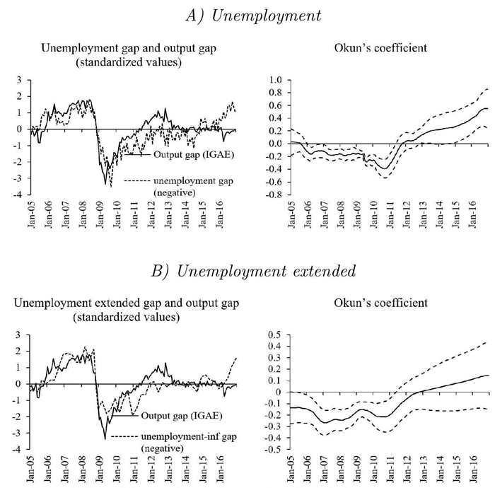
Note: 90% confidence interval. Seasonally adjusted data.
Source: Authors’ calculations with data from INEGI.
Figure 7 Output gap, unemployment gap and Okun’s Coefficient
Despite these differences, all our measures of labor slack seem to be consistent with the economic cycle, i.e., a first period characterized by tightness in the labor market, a post-crisis period with important labor slack, and a reduction in this slack beginning in 2014. In addition, the indicators derived from both indicators of slack show a gradual decrease that becomes more pronounced in the final year, when the unemployment rate is below NAIRU, a difference that is statistically significant. Figure 8 shows the average of all estimations. For the sake of simplicity, in sections 4.3 and 5 we use these averages to analyze employment in the economic cycle with both indicators of labor slack, the traditional measure and the one including informal employment.
4.2 Inflation-predicting performance of each measure of the unemployment gap
In this section, we evaluate the forecasting accuracy of the eight unemployment gaps estimated in the previous subsection. We use the methodology developed by Hansen et al. (2011 that allows us to obtain a subset of superior models for its predictive capacity. The methodology identifies the subset of the models we use that have the best inflation forecasting ability, using the confidence interval acquired through the estimation of a parameter to obtain the model confidence set (MCS) constructed from a predictive equivalence test and elimination rule. This procedure can be summarized as follows: (i) the set of models to be evaluated is chosen in terms of their predictive capacity; (ii) the null hypothesis is that all models have the same predictive ability, while the alternative is that at least one of the models is inferior; and (iii) if the null hypothesis is not rejected, we have a superior set of models. If the null hypothesis is rejected, then the inferior model is removed from the procedure and we return to the previous step. This procedure, unlike other predictive equivalence tests, does not require the choice of a reference model to implement the test.
Specifically, to test whether the models have equivalent predictive performance, Hansen et al. (2011 propose the following test statistic:
where M is the full set of models considered in the predictive evaluation,
The exercises are carried out to evaluate the predictive capacity of the models with different measures of unemployment gaps. This is a pseudo-out-of-sample exercise for different forecast horizons, h = 1,2,...12 , and the average of these horizons. For this exercise, we use the subsample that covers from 2006:12 to 2016:12, with a rolling window of 60 observations.24 The sample for the forecast evaluation considers approximately 35 percent of the full sample (2013:1-2016:12), which corresponds to 48 forecast periods.
Table 2 shows the results of this exercise. Practically all the models for all horizons show an equivalent predictive capacity. A possible exception is the Okun’s law model with the informality unemployment rate that is discarded in some horizons. Thus, the results do not indicate a clear difference in the ability of the unemployment gaps to predict the dynamics of inflation.
Table 2 RMSE and results of the test for predictive ability MCS procedure: T R,M
| Unemployment gaps with respect to the NAURI | Pseudo-out-sample |
|||||||
Variable |
Model |
h=2 |
h=4 |
h=6 |
h=8 |
h=10 |
h=12 |
Average (h=1..12) |
Traditional Unemployment Rate |
Recursive RW RW+AR(2) Okun's law |
0.194 0.192 0.192 0.193 |
0.197 0.195 0.195 0.196 |
0.197 0.196 0.196 0.197 |
0.197 0.195 0.195 0.196 |
0.200 0.197 0.197 0.197 |
0.200 0.197 0.197 0.197 |
0.197 0.195 0.195 0.195 |
Extended measure of Unemplyment |
Recursive RW RW+AR(2) Okun's law |
0.195 0.192 0.194 |
1.98 0.195 0.197 |
0.198 0.196 0.197 |
0.198 0.196 0.197 |
0.210 0.198 0.200 |
0.202 0.198 0.200 |
0.198 0.195 0.197 |
0.196 |
0.201 |
0.201 |
0.199 |
0.199 |
0.198 |
0.198 |
||
Note: The entries shaded in gray represent the models that are elements of the MCS selected by the procedure.
4.3 Measuring inflationary pressures in difficult times
As shown in the previous analysis, there is no clear statistical difference between the two measurements of labor slack in predicting inflation. However, from the policymaker’s point of view, there could be periods when it is especially important to have accurate indicators of inflationary pressures, such as when the unemployment gap is declining and approaching toward zero. Because this type of situation could trigger demand pressures, the policymaker needs the most accurate possible indicator of the unemployment gap. On the other hand, when unemployment is well above the natural unemployment rate, there is little uncertainty that there are no inflationary pressures coming from the labor market.
In this section, we evaluate which labor market slack indicator is more accurate in detecting inflationary pressures when the unemployment gap is close to zero. We use the threshold regression model of the inflation equation that we have used in the previous estimates. The threshold is endogenously estimated in the model. First, as baseline regression we estimate a basic model with no thresholds:
where
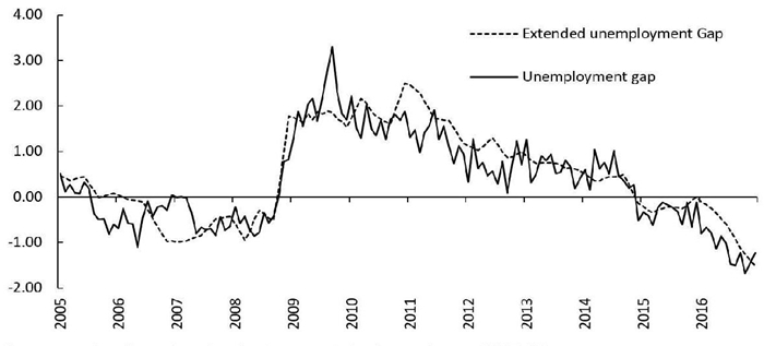
In this subsection, we use the average of the four estimation models for each unemployment measurement. Table 3 shows the results. Column (1) exhibits the results of the traditional unemployment gap, column (2) of the extended unemployment gap, and column (3) shows the results with both unemployment measures in the same equation. When the coefficients of the gaps are estimated separately they are significant and their levels are not statistically different. However, when both measures are included in the inflation specification, their magnitude is reduced by almost half and their standard error more than doubled,25 an obvious indication that the two measures of labor market slack are closely related.26 Figure 9 illustrates the unemployment gaps from the average of the estimates, that is, the gaps calculated from the average estimates of NAIRU-trad and NAIRUinf reported in Figure 8. The gaps are standardized (divided by their standard deviation in the sample) so that their magnitudes can be directly compared. Throughout the sample period the gaps show similar trajectories, but there are some periods with more than subtle differences.
Table 3 OLS estimations of inflation equation
Slack Variables (Slackt) |
Equations |
|||
(Average of the four estimates) |
(1) |
(2) |
(3) |
|
Unemployment gap |
Coeff. (β) |
-0.036 |
- |
-0.018 |
Std. error |
0.009 |
- |
0.021 |
|
t-statistic |
-3.880 |
- |
-0.866 |
|
Extended unemployment |
Coeff. (β) |
- |
-0.034 |
-0.019 |
gap |
Std. error |
- |
0.009 |
0.020 |
t-statistic |
- |
-3.908 |
-0.973 |
|
AIC |
-1.51 |
-1.51 |
-1.50 |
|
BIC |
-1.35 |
-1.35 |
-1.32 |
|
HQIC |
-1.44 |
-1.45 |
-1.43 |
|
R2 Adj |
0.48 |
0.48 |
0.48 |
|
Note: All estimates include two lags of the change in inflation and the change in the annual depreciation of the real exchange rate, plus three pulse dummies for outliers.
Source: Authors’ calculations with data from INEGI.
Source: Authors’ calculations with data from INEGI.
Figure 9 Average estimations of the unemployment gap (standardized values)
We then estimate the threshold regression model. This model allows us to specify a regime change that occurs when a predetermined variable crosses an unknown threshold to be estimated. In particular, we focus on the simplest case of a single threshold (τ ), that is, a model with two regimes described below:
Where
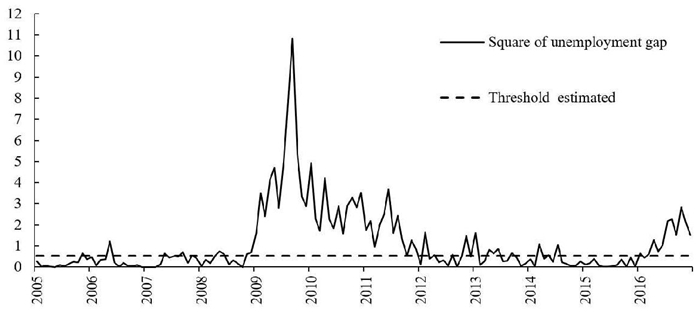
The predetermined variable which helps us to determine the threshold is the square of the traditional unemployment rate gap,
Source: Authors’ calculations with data from INEGI.
Figure 10 Variable of interest to determine the regimes: square of the traditional unemployment gap, τ= 0.52
Table 4 Threshold regression results
Constrains |
||||||
(1) |
(2) |
(3) |
(4) |
|||
Regime |
None |
β1trad=0 ; β2inf=0 |
β1trad= β2trad |
β1inf= β2inf |
||
- |
Coeff. t-Stat. |
- - |
- - |
-0.027 -1.196 |
- - |
|
Unemployment gap |
[1] |
Coeff. t-Stat. |
-0.003 -0.103 |
- - |
- - |
0.130 1.261 |
[2] |
Coeff. t-Stat. |
-0.101 -2.027 |
-0.037 -3.764 |
- - |
-0.013 -.0.592 |
|
- |
Coeff. t-Stat |
- - |
- - |
- - |
-0.026 -1.312 |
|
Extended unemployment gap |
[1] |
Coeff. t-Stat |
-0.034 -1.602 |
-0.043 -2.057 |
-0.021 -1.053 |
- - |
[2] |
Coeff. t-Stat |
0.072 1.3471 |
- - |
-0.001 -0.047 |
- - |
|
|
AIC BIC HQIC formula |
-1.501 -1.274 -1.409 0.485 2.254 |
-1.518 -1.332 -1.442 0.487 0.542 |
-1.498 -1.292 -1.414 0.480 2.173 |
-1.506 -1.300 -1.422 0.484 0.124 |
||
Note: All estimates include two lags of the change in inflation and the change in the annual depreciation of the real exchange rate, plus three pulse dummies for outliers.
Source: Authors’ calculations with data from INEGI.
Column (1) of table 4 shows the result of the non-constrained classical threshold regression model, in which a regime change is permitted in the parameters
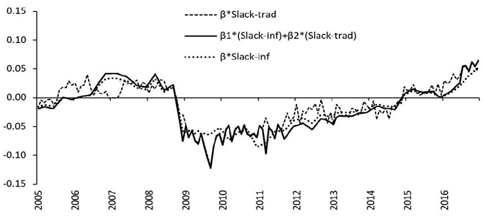
These results might be explained by a period with a high rate of job creation where slack-trad reflects a tight labor market. However, if this period also showed a high rate of low-quality informal labor growth, slack-inf might show a different history, one with a higher level of slack, given that it accounts for this low-quality employment. In such a case, slack-inf could reflect inflationary pressures more accurately.28 The specification of the inflation equation can be decomposed into terms for the determinants of slack, inertia, and supply shocks. In figure 11 we compare the contribution to inflation of the slack components of models (1) and (2) in table 3 with that of the preferred model resulting from threshold regression analysis in table 4. We see that around 2007 the
5. The Mexican labor market over the economic cycle
In this section, we compare the trajectories of slack-trad and slack-inf with the main employment-related economic variables to assess and compare their effectiveness in anticipating demand-driven inflationary pressures. In order to facilitate the analysis, we divide the time span into three periods that take into account the economic cycle in Mexico (figure 12). The first is the pre-crisis period, from 2005Q1 to 2008Q4, which was characterized by inflationary pressures: the GDP gap was positive with the lower bound of the confidence interval close to zero. The second period spans 2009Q1 and 2014Q2, the post-crisis economic slack. The third, from 2014Q3 to 2016Q4, starts with the output gap near zero, and remains close to zero until the end of the study period.
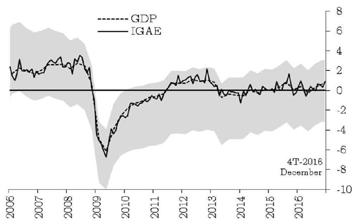
Note: Calculated with seasonally adjusted data. Estimated using the Hodrick-Prescott (HP) filter with tail correction method; see Banco de México (2009: 69). The shaded area is the 95% confidence interval of the output gap, calculated with an unobserved components method.
Source: Calculated by Banco de México with data from INEGI.
Figure 12 Output gap % of potential output; s.a.
We illustrate the main features of the Mexican labor market in each period by describing inflation and monetary policy rates in these periods, and comparing the measures of labor slack with relevant variables such as wages, labor costs, and the GDP gap. Since 2005, there have been two periods of accelerated inflation (2008 and 2017) where Banco de México responded by increasing the reference rate (figure 13). Another event of interest for our analysis is the deflationary period after the worldwide crisis of 2009.
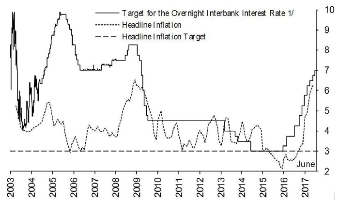
Note: Data before January 20, 2008 refers to the observed Overnight Interbank Interest Rate.
Source: INEGI and Banco de México.
Figure 13 Monetary policy rate and consumer price index % and annual % change
Period I (2005Q1-2008Q4)
During this period, inflation began to pick up (figure 13). The Mexican economy showed some tightness: the GDP gap was positive and statistically significant (figure 12) and wages showed important gains (figure 14d). In addition, unit labor costs in both the manufacturing and service sectors were particularly high throughout this period (figure 14e and 14f).29 However, increases in international food and energy prices also contributed to local inflation (Banco de México, 2008). Slack-inf showed greater tightness than slack-trad, particularly in 2008 (figure 8), which is consistent with the inflationary pressures suggested by other sources of information in the economy. This may indicate that through this period, slack-inf was a better indicator of the Mexican labor market than slack-trad to detect inflationary pressures.
Period II (2009Q1-2014Q2)
During Period II, Mexican economic activity decelerated significantly and went through an important recession as a consequence of the international financial crisis. Wages and labor costs plunged deeply (figures 14d, 14e, and 14f) and are still today far from their pre-crisis levels. Banco de México quickly loosened monetary conditions by decreasing the policy interest rate from 8.25 to 4.5 percent (figure 13). In this period, both measures of slack showed an important increase. However, unlike during Period I, slack-inf suggested a greater degree of slack than slack-trad. Again, it appears that slack-inf better reflected the reality of the Mexican labor market.
Source: Authors’ estimations with INEGI data: ENOE and Economic Information Bank.
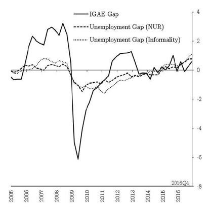
Figure 14 The context of the Mexican labor market A) IGAE gap and the negative of the unemployment gap 1/ %
1/ The IGAE gap is shown as a percentage of the potential output. The negative of the unemployment gap refers to the average estimation for the NAIRU less the observed rate of unemployment.
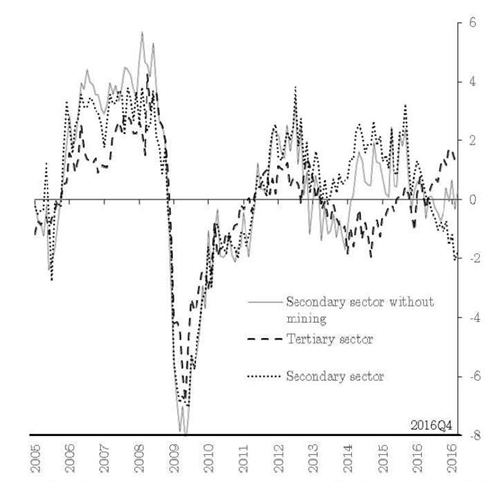
2/ We present the IGAE gap, measured as a percentage of potential output, by sector. Source: Banco de Mexico estimates with data from INEGI.
Figure 15 B) IGAE gap 2/ %, s.a.
3/ Quarterly series. The graph shows the informality rate for the employed population aged 15 or older in urban areas with a population greater than 15,000.
4/ Quarterly data with and without Hodrick-Prescott filter (smooth line, λ=200). Employed population aged 15 or older in urban areas with a population greater tan 15,000. We eliminate wages lower than the 1st and greater than the 99th percentile. When the interviewee did not answer the question about wages with an actual figure, but answered in terms of the minimum wage equivalent, we calculated the monthly wage equivalent.
Source: Authors’ estimations with data from ENOE, INEGI.
Figure 17 D) Average monthly wages of the urban employed population 4/ Real, MXN December 2010
Period III (2014Q3-2016Q4)
Five years after the beginning of the crisis, the slack in the labor market, as measured both by NAIRU-trad and by NAIRU-inf, started declining and continued with this trend until the end of the period (figure 8). At first glance, the latter would suggest the presence of demand-pull inflationary pressures. However, the fact that wages barely grew during this period (figure 14d) and the output gap was still negative suggest no inflationary pressures coming from aggregate demand (figure 14a).
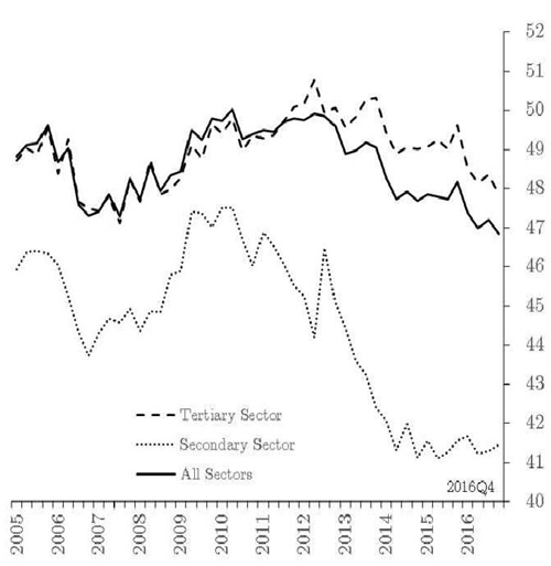
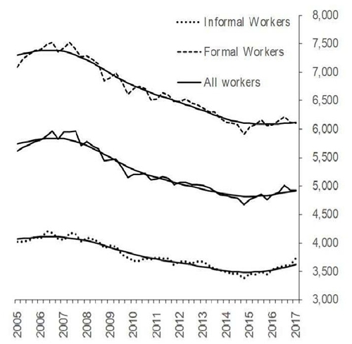
In order to understand this conundrum, we analyze this part of the cycle by separating economic activity in the service and industrial sectors. The slack in the IGAE during Period III is fully accounted for by the negative output gap in the secondary sector (with and without mining) since the end of 2015. In contrast, the tertiary sector (services) output gap closed and crossed into positive territory toward the end of the period (figure 14b). The tertiary sector is also more labor intensive and has a higher level of informal employment than the secondary sector (figures 14c, 14g, and 14h). Finally, the informal sector has considerably lower wages than the formal sector (figure 14d). These three factors provide a plausible explanation of why labor market conditions during this period did not translate into demand-pull inflationary pressures: the service sector, with the highest degree of informal employment and significantly lower wages, was the only productive sector that tightened. Thus, the labor market in Mexico seems to have allowed an adjustment in which workers without formal employment could be absorbed by the service sector into lower-paying jobs, without implying significant inflationary pressures from aggregate demand. During this period, both measures of slack start to suggest tighter labor market conditions. However, once again, slack-inf shows a subtle difference from slack-trad. Figure 8 shows that slack-inf suggests less tightness in the labor market than slack-trad, which is consistent with an absence of wage pressures and lower labor costs, both in the service and industrial sectors.
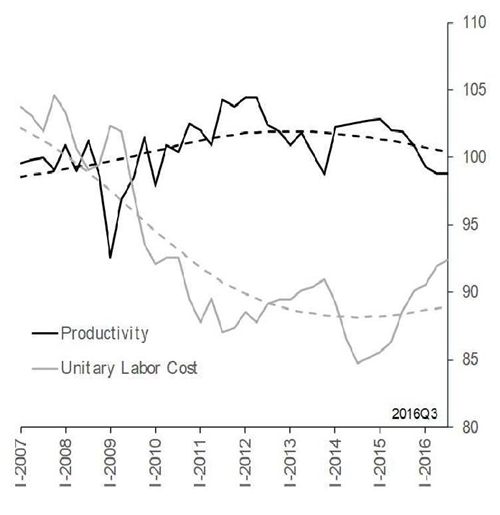
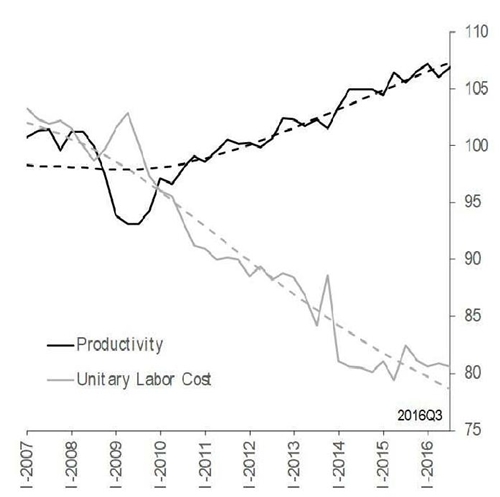
5/ Productivity based on hours worked. Seasonally adjusted series. Trends and seasonal adjustment estimated by Banco de México.
Source: Banco de México using SCNM, ENOE, and INEGI data.
Figure 19 F) Labor productivity and unit labor cost 5/ Services 2008=100, s.a.
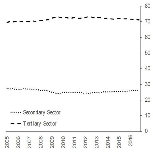
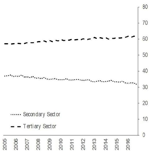
6/ Quarterly data. Employed population aged 15 years and older in urban áreas with a population greater than 15,000. 7/ Using original quarterly series on GDP at 2008 market prices.
Source: Authors’ estimations with INEGI data: ENOE and Economic Information Bank.
Figure 21 H) GDP by Sector 7/ % of total GDP
Finally, it is important to note that Banco de México started tightening monetary policy conditions in December 2015 (figure 13). However, it was emphatic that such pre-emptive policy rate increases were driven by other exogenous shocks at the time (most importantly, exchange rate depreciation) and not by demand-pull inflationary pressures (see Banco de México, 2016).
6. Final remarks
In this study, we estimate two measures of labor market slack for the Mexican economy using traditional NAIRU estimation frameworks. In particular, using traditional methodologies to estimate the nonaccelerating inflation rate of unemployment (NAIRU), we compute two measures of the NAIRU, a traditional NAIRU based on the unemployment rate and an alternative measure (NAIRU-inf), that not only considers the unemployment rate, but also informal wage earners. Our results show no drastic differences in the labor market slack between both indicators over the economic cycle. However, we find subtle differences in some periods. For example, during adverse shocks, differences become significant, since the labor market in Mexico seems to allow an adjustment in which the informal sector can absorb workers without formal employment in lower-paying jobs. During the period of sustained economic growth, informal workers might move to the formal sector, suggesting that the unemployment rate in developing countries with a significant informal labor force could show a relatively lower level and less variation than in advanced economies, where informal sectors tend to be small. With these developments in mind, we propose a complementary analysis of labor market slack using the unemployment rate, with additional information that takes into account the high informality rates that are important in developing economies.
Our results also show that both measures of the NAIRU increased slightly over our study period, and the labor market slack measured with both indicators of labor underutilization showed a similar cyclical pattern. However, consistent with an endogenous threshold model, the slack in the labor market estimated with the indicator including informality seems to predict inflationary pressures more accurately when the unemployment gap is close to zero. For example, slack-inf better anticipated the inflationary pressures observed in 2007-2008. In addition, during 2016, this alternative measure showed a greater degree of slack than the traditional one, which is consistent with the absence of considerable wage pressures observed during this period.
We do not suggest replacing the use of the traditional labormarket slack indicator (slack-trad) with the indicator that includes informal employment (slack-inf) for analytical purposes, but we do propose using it as an additional measure to complement the analysis. First, economic situations may be exposed to diverse factors at different times: a particular situation, for example, could lead to an overweighting of a specific slack indicator. Second, slack-trad is calculated with monthly data, while slack-inf is calculated quarterly. Thus, slack-trad offers policymakers a timelier indicator of labor market slack than slack-inf, since monetary policy decisions are made approximately every month and a half.
Finally, we consider that the subtle differences between the indicators identified in this paper may be useful for policymakers evaluating labor conditions at a particular moment in time, particularly when the unemployment gap is close to zero. We conclude that the inclusion of informal employment can complement the analysis of the Mexican economic cycle and can be a useful tool for monetary policy formulation not only in Mexico, but also in other developing countries.