


 text new page (beta)
 English (pdf)
 Article in xml format
 Article references
 Send this article by e-mail
 Cited by SciELO
  Similars in
SciELO
Similars in
SciELO 
 Permalink
1. Introduction
Due to their potential impact on a society's welfare and economic growth, several studies have examined microfinance institutions (MF Is). Another reason for this interest is that MFIs represent an oppor-tunity to achieve financial inclusion and eradicate poverty and have therefore become an essential part of one of the United Nations development goals (Patino, 2010).
"If the interest rate increase becomes important, evidently, we will have to follow the market, funding costs for us will increase too, and evidently, we could have a scenario with higher-cost loans-", Patricio Diez, Gentera Group CFO (Juárez, 2016). The previously quote comes from an article published by a Mexican newspaper in re-sponse to the 2016 interest rate increases announced by Mexico's Cen tral Bank, which occurred both in Mexico and other emerging market economies, caused by an increase in US interest rates. These increases were significant because some institutions, particularly MFIs, were already charging high interest rates. For instance, the Mexican MFI Gentera Group had an average interest rate of 65% in 2015.1 One of the primary concerns about MFIs is the dramatic difference in mi-crocredit interest rates by region and country. For instance, while there is evidence of MFI interest rates of around 20-22% in countries such as India and Bangladesh, in Mexico and some African countries interest rates have been as high as 100% (MIX Market Intelligence, 2015). The main reasons for these differences seem to be country-specific (Kneiding and Rosenberg, 2008). In graph 1, we show the mean interest rate per country and variations among interest rates to reveal the dimension of the variability within and among countries. There are many points well above and below these countries averages, and Mexico's mean is seen to be above the other countries sampled.

Source: Authors' own.
Note: circles represent outliers and asterisks represent extreme outliers.
Graph 1 Boxplot of interest rates in MFIs per country
The significant differences in MFI interest rates among countries and regions is not new; however, as far as we know, it has not been deeply studied. In this paper, we contribute to the literature by analyzing the factors that explain these large variations. We also answer the question of whether these differences are explained by internal variables or by the external environment in which they develop. In particular, we study MFIs from Latin America, Africa, Eastern Europe and Asia. In this regard, Campbell (2010) found that microcredit interest rates were below consumer-credit interest rates in Asian countries, while in Latin America and African countries it was the op-posite, with microcredits being more expensive than consumer credit.
Few studies have analyzed interest rates specifically for MFIs, and most of them do so with a single level analysis. Although their findings are quite relevant for the field, we believe that it is essential to go further and review those findings with new tools. In this case, a sig nificant contribution of this work is the use of a multilevel approach, which allows us to understand the variations in interest rates within and among countries and regions. In this regard, Hitt, Beamish, Jackson and Mathieu (2007) found that a single-level analysis cannot wholly explain world problems, because they are complex multilevel phenomena. They argue that multilevel models are thus more useful for analyzing these kinds of issues. In this study, we use Hierarchical Linear Modeling (HLM), which is a multilevel model. This type of model considers individual- and group-level variations, among other features, when estimating group-level regression coefficients. Also, HLM allows us to relax the assumption of heteroscedasticity in error terms, which is a crucial assumption of linear models like OLS.
Our methodology is similar to that of Sun and Im (2015), who also used a multilevel model, combining MFI interest rates with coun-try-level variables to analyze interest rate determinants. The dif-ference between their study and ours is that their focus was on en-trepreneurship, with a co-creation perspective. Our study focuses on internal and external variables that may affect interest rates at MFIs. Another contribution of this paper is the incorporation of variables related to the perception of government effectiveness, to explain in terest rate differentials among MFIs in different countries.
We organize the remainder of this paper as follows. The second section presents a brief literature review and a theoretical framework. The third section describes the data and methodology. The fourth section discusses conclusions.
2. Literature review theoretical framework
2.1. Literature review on interest rate in MFIs
The debate on microfinance interest rates started in the 90s when in-stitutionalists claimed that credit demand was inelastic to changes in interest rates, and they argued that subsidies could be eliminated and that MFIs should achieve sustainability,2 by charging higher interest rates (Kar and Bali Swain, 2014). Morduch (2000) introduced the term microfinance schism, which describes the conflicting objectives in MFIs in their efforts to continue serving the unbanked sector: to fight for poverty reduction or to focus on profitability. Many studies have focused on investigating whether this schism exists or not (Cotler and Rodríguez-Oreggia, 2008; Bos and Millone, 2015; Vanroose and D'Espallier, 2012; Kar, 2013; Balammal, Madhumathi, and Ganesh, 2016), while some others have focused on finding the determinants of interest rates (Cotler and Almazan 2013; Roberts, 2013; Dorfleitner, Leidl, Priberny, von Mosch, 2013; Basharat, Hudon, and Nawaz, 2015; Guo and Jo, 2017). However, none of these studies have been able to definitively explain the variability in interest rates among countries and regions.
Sun and Im (2015) took a stakeholder approach and assessed the proportion of female borrowers, the proportion of loan executives, and the role of governments in the MFIs, all of which were MFI-level variables, and used other country-level variables as a control. The only country-level variable used as an independent variable in their study was the measure of rule of law. They found that interest rates tend to be lower in countries with a higher degree of rule of law.
Other studies that provide some clues about the reason for the variance in interest rates have focused on mission drift and financial development. For example, Cotler and Almazan (2008) reported that interest rates in Mexico were almost double of those of other Latin American MFIs. Although it was not their purpose to explain this variability, they found that high-interest rates were a consequence of the youth of Mexican MFIs.
Regarding the studies that justify interest rate determinants, Bogan (2012) found evidence that MFIs charge high-interest rates to protect their investment from a lack of collateral to secure their loans. Cotler and Almazan (2013) studied the core drivers of interest rates. They found that funding costs, loan size and efficiency levels, measured by operating expenses, were crucial to determining interest rates. They used competition as a country-level variable and proved it using simultaneous equations. However, this approach does not provide a measure of variability. They concluded that an increase in competition leads to a reduction in interest rates and in the average loan size.
On the other hand, Roberts (2013) found that, although market competition should force MFIs to become efficient and decrease their interest rates, the behavior in for-profit MFIs was different, as they tend to impose higher effective interest rates compared to other MFIs, despite a more competitive environment. Furthermore, he found that for-profit institutions tend to have higher interest rates for their bor-rowers than non-profit institutions. Dorfleitner, Leidl, Priberny and von Mosch (2013) found that operating expenses were the most cru cial variable in determining interest rates. They also found evidence that interest rates for female borrowers are higher than male ones, and that regulated MFIs tend to charge lower interest rates than un-regulated ones. Vanroose and D'Espallier (2012) found a negative relationship between financial sector development and the financial performance of MFIs. They concluded that competition with banks might force MFIs into one of two possible outcomes: serving poorer customers (thus increasing their costs) or reducing their interest rates to compete with banks.
Other studies that indirectly analyze MFIs' interest rates include the one of Cull, Demirgüc-Kunt and Morduch (2014). They ex-plored the impact of bank penetration in the financial development and found a negative relationship between bank penetration and the interest rates; this result reinforces the argument of Vanroose and D'Espallier (2012) concerning the increased possibility of find more developed MFIs in a more highly developed financial system. Com-plementing this finding, Trujillo, Rodriguez-Lopez, and Muriel-Patino (2014) found that in more developed regulatory environments, espe-cially those with strong supervisory practices, MFIs interest rates tend to be lower. Xu, Copestake and Peng (2016) found that the smaller the loans of the MFIs, the larger the interest rates.
Regarding the profitability, profit margins and interest rates of MFIs, Kar and Bali Swain (2014) showed that higher interest rates in-crease the profitability of MFIs. Recognizing this premise, Nwachukwu (2014) analyzed this relationship and showed that the idea is valid only up to a certain point; thus, there is a U-shaped relation between interest rates and profitability; she found a 76% as the inflection point.
In another study, Kar and Bali Swain (2014) found that a more competitive environment will cause interest rates to increase and recommend regulatory measures to counteract the adverse effects. In that study, just like in ours, they used the Boone indicator as a mea-sure of the degree of competition.
In 2016, Cuellar-Fernandez, Fuertes-Callen, Serrano-Cinca, and Gutierrez-Nieto analyzed margins in microfinance institutions. They found that operating expenses are the primary factor in explaining margins and that MFIs who operate in countries with higher financial inclusion have lower margins. Also, they discussed the concept of "poverty penalty", which holds that the poorer customers who pursue smaller loans generate higher margins for MFIs.
2.2. Theoretical framework
As we mention before, in this work we try to explain the variability in interest rates in some countries, using the real yield on the gross loan portfolio as a proxy for the interest rate. In this section, we explain the causal link between the identified explanatory variables and interest rate. Also, we explain the relevant hypotheses of this paper regarding the explanatory variables. To this end, we explain first the MFI-level variables, and then the country-level variables.
The first MFI-level explanatory variable is average loan balance per borrower, the amount of money borrowed from MFIs per borrower.
With regard to this variable, Kneiding and Rosenberg (2008) found that one of the primary drivers of higher interest rates is small loan sizes, and argue that reaching poorer customers, who make smaller loans, is more expensive. Other authors, such as Navajas and Tejerina (2006), Sun and Im (2015), Basharat, Hudon and Nawaz (2015), Xu, Copestake and Peng (2016), and Cuellar-Fernandez, Fuertes-Callen, Serrano-Cinca, and Gutierrez-Nieto (2016) also analyzed the relation-ship between average loan balances and interest rates, and found a negative correlation between these two variables as well. For Mexican MFIs, the ProDesarrollo (2014) annual report found a similar result. Thus, in this article, we expect to find that the smaller the amount of the loan, the higher the interest rate.
The second MFI-level variable is operating expenses as a proportion of total assets. In this work, we expect to find a positive relationship between operating expenses and interest rates because, according to Dorfleitner, Leidl, Priberny and von Mosch (2013), operating expenses are the primary drivers of interest rates, so in order to stay solvent MFIs must increase interest rates when their expenditures increase.
Our third variable is the age of the MFIs. We include this variable because some empirical studies have found that mature MFIs tend to be more efficient, and that they gain efficiency by reducing information asymmetries and taking advantage of economies of scale (Cuellar-Fernandez, Fuertes-Callen, Serrano-Cinca, and Gutierrez-Nieto, 2016). This allows them to reduce the interest rates faced by their borrowers. Other studies have found that, in order to reduce risk, younger MFIs tend to lend to wealthier customers (Xu, Copes-take and Peng, 2016). Because of these arguments, we expect to find a negative relationship between the age of the MFI and the interest rate they charge. As a proxy for this variable, we use a categorical variable that indicates the longevity of the MFI, classified in one of the three groups: new (one to four years in business), young (five to nine years in business) and mature (more than nine years in business).
The fourth MFI-level variable is the portfolio at risk. This variable represents the value of all outstanding loans that have payments that been due for more than 30 days, divided by the gross loan port folio, expressed as a ratio. For this variable, we have different argu-ments concerning the impact of this variable on the average interest rate charged by an MFI. On the one hand, Nwachukwu (2014) found that MFIs with higher proportions of the loan portfolio at risk tend to charge higher interest rates. On the other hand, Sun and Im (2015) claimed that it is a common practice in MFI industry to renegotiate debts, which in many cases implies lowering interest rates to promote repayment. For this article, our hypothesis for this variable is in the sense of Sun and Im (2015), the higher the portfolio at risk, the lower the interest rate the MFI charges to customers.
The last MFI-level variable is legal status of the MFIs: whether the MFI operates as a nonprofit or for-profit institution. In the literature on this subject, Cull, Demirgüc-Kunt, and Morduch (2009) found that non-profit MFIs tend to charge higher interest rates due to their higher operating costs.
We use three country-level variables: government effectiveness, degree of market competition and real GDP. Government effectiveness is related to the country or political risk; this risk is associated with the degree of uncertainty with respect to the stability of the political and economic system (Reilly and Brown, 2012). We expect this vari able to have a positive relationship with the interest rate, since we expect that interest rates will increase when perceived risk increases. The real growth GDP is the most common measure of a country's overall economic activity. We expect to find a positive relationship between real growth GDP rates and interest rates, because according to Cull, Demirguücc-Kunt and Morduch (2014), countries with higher GDP growth rates tend to have a higher bank penetration, forcing MFIs to increase interest rates to attend the poorest.
Finally, we include an indicator of competition, the BOONE indicator, following the study proposed by Kar and Bali Swain (2018). We expect to find a positive relationship between the BOONE indi-cator and interest rates because according to those authors, MFIs located in a more competitive environment have greater incentives to increase interest rates, to obtain sufficient resources to spend on increasing their market share. In this regard, the BOONE indicator, also known as "profit-elasticity", is measured through the elasticity of profits to marginal costs. An increase in the BOONE indicator implies a weakening of financial intermediaries, which means that a competitive environment punishes inefficient institutions, including MFIs. According to these authors, there are other indicators for the degree of competition, such as the Lerner index and the H-Statistic. However, these indicators fail to measure competition in loan markets, because of interest rate regulations.
3. Data and methodology
For this study, we use Hierarchical Linear Modeling (HLM). This model allows for heteroscedastic error variance. In this regard, a critical assumption of linear methodologies like OLS is the Independence of the error terms or homoscedastic error variance. However, clus-tering of observations within groups leads to correlated error terms, biased parameters, and standard errors. Adjusting for this variability in the error variance is a central point of HLM (Garson, 2013). Another essential feature of HLM is that the coefficients are not inter-preted as fixed, as in OLS. Instead, they are considered as a variable, formed with a fixed term and an aleatory component; allowing the separation of within-group and between-group effects (Pardo, Ruiz and San Martín, 2007). Furthermore, according to Hitt, Beamish, Jackson and Mathieu (2007), HLM is the proper tool to analyze problems in management because it provides more exact estimations of data, since it can be used to work with distinct levels.
According to Gelman and Hill (2006), there are three main fea-tures that distinguish the coefficients of HLM from those of classical regressions: i) they can vary according to group; ii) they can have more than one variance component; and as a result, iii) they can be different depending on whether they are estimated individually or across groups. In this work, we are interested in estimating variation in interest rates for countries of Latin America and Asia.
To use HLM, we first need to set up a regression with varying coefficients, and then set up a regression for the coefficients themselves (Gelman and Hills 2006). As proven by Gaviria (2000), HLM is a particular case of a Structural Equation Model, wherein the maximum likelihood estimators belong to a parameter that depends on non-observable variables. In this work, the model is solved through the EM algorithm proposed by Dempster, Laird and Rubin (1977). HLM can also be used to analyze data with sophisticated patterns and nested sources of variability (Castro and Lizasoain, 2012). In this regard, our database (Mix Market Intelligence) is a good candidate for HLM analysis, because it has an inherent multilevel structure with many data points per MFI, and because we also grouped MFIs into countries and countries into regions.
The database contains information from 962 MFIs, grouped into 25 countries and five regions, from 2009 to 2015. It is important to note that not all countries have the same number of observations, and not all MFIs reported data during the entire period (see appendix 1). For example, while most MFIs reported data for only three years, many of them did report data in the period analyzed. Thus, we have different numbers of observations per group; in this regard, HLM gives more weight to groups with more observations (Huta, 2014).
The idea behind HLM is that if an individual, an MFI in this case, belongs to one country/region, then the context in which they develop is different. The model also captures whether MFIs share specific characteristics, which at a certain level makes them homogenous within countries and heterogeneous between countries. Thus, instead of analyzing each of their respective contexts, HLM allows for differ-entiating the variability at each level with one single model (Castro and Lizasoain, 2012).
As an example how HLM works, see graph 2, where the scat-terplot shows the trending lines for three selected countries. Each point reflects the intersection between Real Yield and Operating Ex pense in Mexico (o), Bangladesh (■) and Perú (x). In the graph, we see that the trending line appears to have a slightly different slope and different intercepts for each of these countries. This means that the relationship between operating expenses and interest rates is not the same in all countries; by using HLM, we were able to find these relationships.
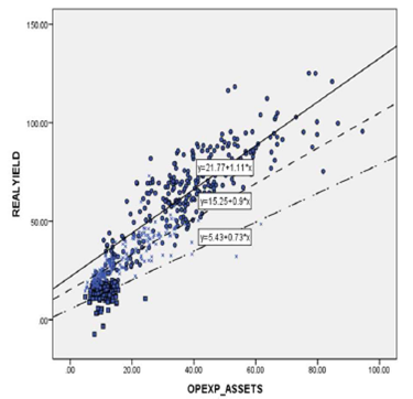
Source: Author´s own, base don infotmation from the MIX Market Intelligence detabase
Graph 2 Trending lines of the relation between operating exprenses and interest rates
In this paper, we follow the methodology proposed by Pardo Ruiz and San Martin (2007). According to this methodology, we first need to use a null model to compare the results. Then, we analyzed the means and covariance's followed by an analysis of random coefficients, which gave us an integrated model with random coefficients and slopes.
3.1. Statistical analysis of the data
The database was randomly selected to cover methodological require-ments. We selected countries with more than 100 observations and eliminated those MFIs with significant missing information. As a re-sult, our sample contains 25 countries and five regions (see appendix 1). Next, we standardized the data according to international ac-counting standards to make the data comparable (Cull Demirguücc-Kunt and Morduch, 2009). We also took some variables from the World Bank Database (World Bank, n.d.(a)) and the World Gover-nance Index (World Bank, n.d. (b)). Table 1 contains a brief description of the variables used in this work.
Table 1 Definition of variables
| Variables | Short name |
| Real yield on gross loan portfolio | REALYIELD |
| Government effectiveness+ | KKM |
| Real growth GDP++ | GDP_REALGROWTH |
| Boone indicator as a measure | BOONE |
| of competitionH++ | |
| Average loan per borrower, as | LOANBORR-GNI |
| proportion of GNI per capita | |
| Operating expenses | OPEXP_ASSETS |
| Age of the microfinance institution | AGE |
| Profit orientation (profit or non-profit) | PROFITSTATUS |
| Portfolio at risk witliin 30 days | PAR30 |
Note: +World Governance Indicators database from World Bank (n.d.(a)), +-+World Development Indicators database from World Bank (n.d.(b)).
Appendix 2 contains a brief descriptive statistic for the variables in table 1, where the statistic Valid N (listwise) indicates the number of useful observations that matched all items, which in this case is 3,182. We see that on average MFIs charge an interest rate of 23.4%, with an 18.5% standard deviation. Another interesting statistic in appendix 2 is the correlation between real yield and average loan per borrower (as a proportion of GNI), which is negative. This result means that the smaller the loan, the higher the interest rate. Finally, we see a high correlation between operating expenses and interest rates, which is consistent with previous studies about the primary drivers of interest rates (Dorfleitner Leidl, Priberny and von Mosch 2013).
3.2. Null model: Country as random factor
In this section, we run a model called the null model. This model helps us to verify the degree of variability among the countries in our analysis. As a result, we obtain the Likelihood Ratio, which is used to compare the different estimated models. This ratio helps to verify whether the proposed models fit in multilevel analysis. In this case, this null model addresses the question: is there a level 2 country effect on the level 1 intercept of the interest rate? If there is a country effect, the linear models like OLS will suffer from correlated error, and some form of linear mixed modeling is required (Garson, 2013).
It is important to note that the null model is the shortest mul-tilevel model. In this model, there are no explanatory variables, only the dependent variable, the first level variable, and two unobserved random effects. In our case, the null model is the following
Where sub-index i represents the MFI, and j is the country. Thus REALYIELDij is the interest rate of MFI i in country j, p0 is the overall mean of interest rates among countries, u 0 j is the effect of the country and eij is an MFI-level residual. As in OLS, in this null model we assume that uoj and eij are aleatory variables with zero mean and a constant variance.
To estimate the model, we use Stata xtmixed command with max imum likelihood estimation (ML). We could have used the restricted maximum likelihood (REML) instead, but this method does not allow for the comparison of different models using the likelihood ratio test. Also, according to Snijders and Bosker (1999), in large samples the differences in the results between these two methods are negligible. Another advantage of the xtmixed command is that it belongs to a broader class of commands used to estimate models with longitudinal data (Albright and Marinova, 2010), as in this work.
We show the results of equation (1) in the first column of table 2. As we expected, we found a mean interest rate of 23.67%, which we use as an estimator of the mean population. Nevertheless, the main result from the null model is the interclass correlation coefficient (ICC), which is estimated as follows:
This coefficient means the proportion of country-level variance, Var(u 0j ), from the total variance, where Var (e ij ) is the MFI-level variance. Regarding the ICC coefficient, there is a debate around whether a significant ICC validates the use of HLM since this model allows uncorrelated errors, which is an assumption that models like OLS do not allow (Roberts, Monaco, Stovall, and Foster, 2011). However, in this work, we interpret the ICC coefficient as the degree of dependence of individuals upon a higher structure to which they be-long (Roberts, Monaco, Stovall, and Foster, 2011). In our sample, the ICC is 51%; in this case, this is the variation of the interest rate attributable to a country characteristic. In this regard, ICC could be evidence that using multilevel models is appropriate; whether the intercept of the null model is significant, the ICC coefficient is also significant, and HLM is appropriate (Garson, 2013), which is the case for our data (see the first column of table 2).
3.3. Mean analysis
Now that we have some evidence that variations in interest rates are attributable to a country characteristic, the next step is to verify whether variations within and between countries could be reduced with each of the country-level variables. The first level model is:
The second level model, which interacts with one of the country-level variables, is:
Combining both we get:
For this work, X
j
is each of the following variables: KKM, GDP_REALGROWTH or BOONE, in each of the models. The coefficient Yoo is interpreted as the average interest rate for the entire population, while Ycn becomes the estimator of each Xj, and as usual measures the effect of each independent variable on the dependent one. Next, u0j- is the unobserved effect of each country after con-trolling for the variable Xj. In this model, u
0j
and eij are random variables. Note that the parameter
Table 2 Results of equation 5
| Null model | Mean analisys | |||
| Coef. (SE) | Coef. (SE) | Coef. (SE) | Coef. (SE) | |
| Constant | 23.67*** | 25.1*** | 23.59*** | 24.16*** |
| (2.27) | (2.38) | (2.28) | (2.27) | |
| KKM | 3.096* | |||
| (1.86) | ||||
| GDP_REALGROWTH | 0.035* | |||
| (0.02) | ||||
| BOONE | 2.44* | |||
| (1.08) | ||||
| var (-cons) | 127.97 | 121.8 | 128.5 | 132.33 |
| (36.39) | (34.78) | (36.54) | (36.94) | |
| var (Residual) | 126.3 | 126.25 | 126.19 | 132.75 |
| (2.95) | (2.95) | (2.95) | (2.93) | |
| N | 3693 | 3693 | 3693 | 3693 |
| Years | 7 | 7 | 7 | 7 |
| Countries | 25 | 25 | 25 | 25 |
| ICC | 0.51 | 0.49 | 0.50 | 0.50 |
| Log Likelihood | -14235.26 | -14233.89 | -14233.71 | -15948.82 |
Source: Author's own. Note: *significant at 90%, **significant at 95%, ***significant at 99%.
As we can observe in table 2, all the variables are significant, which implies that all of them are good estimators of the independent variable. Furthermore, the variance of these coefficients is smaller than the variance of the null model, var (cons). On the other hand, if we compare the variance in each country, var (Residual), against the variance of the null model, it decreases for all variables, except for the BOONE indicator, which means that these three variables explain a significant portion of the interest rate variation. As a test of goodness of fit, we use the likelihood ratio: the lower the ratio, the better the goodness of fit (Pardo, Ruiz and San Martin, 2007). As can be seen in table 2, except for the BOONE variable, the three variables are good estimators for the interest rate. In addition, the log likelihood associated with each variable is smaller than that of the null model, and is almost constant, which indicates that intra-country variance remains the same.
3.4. Covariance analysis: one random effects factor
In the last section, we analyzed variations of level 2 (country-level) variables. In this section, we add the level 1 variables, MFI level variables, to examine the differences in MFIs from the same country via a covariance analysis, which aims to explain the within-country variance. To test whether each variable reduces the variability and improves the model fit, for this model we add the MFI-level variables one by one, combined with each country-level variable. In this case, we add the variables: LOANBORR-GNI, OPEXP_ASSETS, AGE, PROFITSTATUS and PAR30.
For example, for the case OPEXP_ASSETS and KKK the model is: REALYIELDij = Po + Pij
Where
Combining them we obtain:
We show the results of equation (8) in table 3. Since the ICC is a conditional coefficient it explains the proportion of the total variance that is due to the MFI-level variables. After controlling for MFI-level variables, the proportion of the variability in interest rates due to the country features can be seen. The more the ICC decreases, compared to the null model, the more the differences observed within countries are explained by the variability in each of the MFl-level variables (LOANBORR_GNI, OPEXP_ASSETS, AGE, PROFITSTATUS). As we can see in table 3, for any combination of MFI and country variables, the ICC is smaller, especially in the case of operating expenses. The ICC coefficient remains almost constant when we add the variables LOANBORR_GNI and PAR30.
The degree of variability within countries is explained by the statistic var (Residual). In all cases, the statistic var (Residual) is smaller after adding level 1 variables than in the null model, which means that the combinations of MFI-level and country-level variables are explaining a significant portion of the within-country variability. Another relevant result is that for all combinations, all the coefficients are significant, except for the profit status. Furthermore, the likeli-hood ratio shows that for all combinations each variable is a good estimator of the interest rate; which is a goodness of fit test.
Table 3 Covariance analysis
| Coef. | Coef. | Coef | Coef | Coef | Coef | Coef | Coef | Coef | Coef | |
| (SE) | (SE) | (SE) | (SE) | (SE) | (SE) | (SE) | (SE) | (SE) | (SE) | |
| 1 | 2 | 3 | 4 | 5 | 6 | 7 | 8 | 9 | 10 | |
| Constará | 26.61*** | 11 77*** | 30.88*** | 25.517*** | 26.18*** | 24.79*** | 10.52*** | 29.29*** | 24.06*** | 24.31*** |
| (2.36) | (1.5) | (2.48) | (2.39) | (2.4) | (2.27) | (1.4) | (2.36) | (2.29) | (2.31) | |
| KKM | 3.74** | 2.54* | 3.001* | 2.96 NS | 3.81** | |||||
| (1.83) | (1.39) | (1.79) | (1.82) | (1.9) | ||||||
| GDP_ REALGROWTH | 0.039** | .036** | 0.0278 NS | 0.028 NS | 0.05** | |||||
| (.02) | (0.016) | (0.019) | (0.019) | (0.022) | ||||||
| BOONE | ||||||||||
| LOANBORR-GNI | -0.016*** | -0.016*** | ||||||||
| (0.001) | (0.001) | |||||||||
| OPEXP-ASSETS | 0.773*** | 0.773*** | ||||||||
| (0.015) | (0.015) | |||||||||
| AGE | -2.075*** | -2.03 | ||||||||
| (0.333) | (0.333) | |||||||||
| PROFITSTATUS | -0.29 NS | -0.29 NS | ||||||||
| (0.44) | (0.44) | |||||||||
| PAR30 | -0.056*** | -0.055*** | ||||||||
| (0.01) | (.011) | |||||||||
| var (-cons) | 119.99 | 43.74 | 118.003 | 127.75 | 123.04 | 127.38 | 46.55 | 123.77 | 133.66 | 131.78 |
| (34.23) | (12.58) | (33.07) | (35.82) | (35.17) | (36.22) | (13.33) | (34.55) | (37.33) | (37.51) | |
| var (Residual) | 118.24 | 74.3 | 113.991 | 132.41 | 121.3 | 118.19 | 74.23 | 133.97 | 132.39 | 121.191 |
| (2.83) | (1.75) | (3.007) | (2.99) | (3.01) | (2.82) | (1.75) | (3.007) | (2.99) | (3.01) | |
| N | 3625 | 3625 | 3625 | 3269 | 3532 | 3625 | 3625 | 3625 | 3269 | |
| Years | 7 | 7 | 7 | 7 | 7 | 7 | 7 | 7 | 7 | 7 |
| Countries | 25 | 25 | 25 | 25 | 25 | 25 | 25 | 25 | 25 | 25 |
| ICC | 0.5 | 0.37 | 0.51 | 0.49 | 0.50 | 0.52 | 0.39 | 0.48 | 0.50 | 0.52 |
| Log Likelihood | -13499.99 | -13005.57 | -15513.13 | -15281.79 | -12539.45 | -13500.1 | -13004.58 | -15513.53 | -15282.09 | -12538.89 |
| 11 | 12 | 13 | 14 | 150 | |||
| Constará | 25.55*** | 11.06*** | 29.80*** | 24.37*** | 25.02*** | ||
| (2.28) | (1.42) | (2.39) | (2.31) | (2.32) | |||
| KKM | |||||||
| GDP_REALG ROWTH | |||||||
| BOONE | 2.49* | 2.55*** | 2.82* | 2.27* | 2.70* | ||
| (1.06) | (0.85) | (1.10) | (1.11) | (1.10) | |||
| LOANBORR-GNI | -0.016*** (0.001) | ||||||
| OPEXP-ASSETS | 0.78*** (0.014) | ||||||
| AGE | -2.08 (0.333) | ||||||
| PROFITSTATUS | -0.29 NS (0.411) | ||||||
| PAR30 | -0.054*** (.011) | ||||||
| var (-cons) | 132.97 | 49.81 | 126.26 | 135.94 | 137.59 | ||
| (37.11) | (14.01) | (35.26) | (38.00) | (38.44) | |||
| var (Residual) | 123.46 | 78.51 | 133.81 | 132.30 | 125.85 | ||
| (2.8) | (1.75) | (3.00) | (2.99) | (2.98) | |||
| N | 3532 | 3625 | 3625 | 3625 | 3269 | ||
| Years | 7 | 7 | 7 | 7 | 7 | ||
| Countries | 25 | 25 | 25 | 25 | 25 | ||
| ICC | 0.52 | 0.39 | 0.49 | 0.51 | 0.52 | ||
| Log Likelihood | -15041.98 | -14585.46 | -15511.26 | -15280.99 | -13842.77 | ||
Source: Author's own. Note: *significant at 90%, **significant at 95%, ***significant at 99%.
3.5. Random coefficients analysis
In the previous sections, the relationship between MFI-level variables and interest rates is assumed to be homogeneous among all countries. However, to verify which part of the intra-class variance is explained for the independent MFI-level variables, we evaluated each country equation, and then examined how the intercepts and slopes vary in each country. This model is called the random coefficients model because it allows intercepts and slopes to vary randomly per country. For example, for the case OPEX_ASSETS the model is:
Where
Where γ 00 characterizes the mean interest rate across countries, 𝛾 10 is the mean slope which links operating expenses and interest rates, u0j- is the effect of each country on the means, and u 1j is the effect of each country on the slopes. In table 4, we show the results of equation (10). Again, all coefficients were significant. In this model, the likelihood could be used to test random slopes.
Table 4 Random coefficients analysis
| Coef. | Coef. | Coef. | Coef. | Coef. | |
| (SE) | (SE) | (SE) | (SE) | (SE) | |
| Constant | 26.68*** | 11.19*** | 29.44*** | 23.16*** | 25.29*** |
| (2.65) | (1.04) | (3.14) | (2.10) | (2.42) | |
| LOANBORR_ GNI | -0.095*** (0.032) | ||||
| OPEXP_ASSETS | 0.68*** (0.067) | ||||
| AGE | -2.01*** (0.77) | ||||
| PROFITSTATUS | 1.88 N8 (2.15) | ||||
| PAR30 | -0.18*** (0.04) | ||||
| var (slope) | 0.025 | 0.1025 | 9.91 | 100.15 | 0.022 |
| (0.007) | (0.031) | (4.86) | (34.65) | (0.013) | |
| var (intercept) | 173.75 | 23.48 | 214.37 | 108.90 | 144.65 |
| (49.5) | (7.47) | (69.69) | (31.39) | (41.29) | |
| covar | -1.78 | -0.32 | -30.04 | -11.53 | -0.92 |
| (slope, intercept) | (0.56) | (0.37) | (15.72) | (22.61) | (0.51) |
| var (Residual) | 100.23 | 63.61 | 132.32 | 123.45 | 118.54 |
| (2.4) | (1.5) | (2.98) | (2.80) | (2.96) | |
| N | 3532 | 3625 | 3625 | 3625 | 3269 |
| Years | 7 | 7 | 7 | 7 | 7 |
| Countries | 25 | 25 | 25 | 25 | 25 |
| Proportion of | 21% | 50% | 0.5% | 7.1% | 6% |
| explained variation | |||||
| Log Likelihood | -13253.27 | -12751.08 | -15504.894 | -15175.955 | -12514.22 |
Source: Author's own. Note: *significant at 90%, **significant at 95%, ***significant at 99%.
In this section, we analyze each of the variance components, since they represent the main findings in this model. First, to test whether the variance of the slope is significant, we need to verify whether the coefficient is more than three times the standard error (Leckie, 2010). The results in table 3 show that LOANBORR_GNI and OPEXP_ASSETS have random intercepts and random slopes. A significant random slope means that the effect of the average loan per borrower, or operating expenses, on the interest rate is not the same for each country, as described in graph 1. Using the predicted values obtained with OPEXP_ASSETS, we obtain the lines shown in graph 3. Each line represents a different country, and we can observe how the slopes and the intercepts of each regression line are different.
In equation (10), the covariance is an indicator of the relation between slopes and intercepts. In the case of the variables OPEXP_ASSETS and PAR30 the relationship with interest rates keeps on after the changes in the means; this indicates that in this case, there is no statistical evidence of a link between slopes and intercepts.
Finally, the residual variance shows the variability of each MFI around its country regression line, and it allows us to assess the variable that explains most of the variation within a country; in this case, the variable operating expenses has the greatest variation.

3.6. Integrated model: random coefficients and slopes
In the previous sections, we established that the eight out of the nine variables tested were significant interest rate predictors; we could not find statistical significance for the variable profit status. We also verified that these variables explain a significant proportion of the variability among MFIs and countries. Now, to evaluate why real interest rates are higher in some countries than in others and why the relation between MFI-level variables and interest rates is different in each country, we need to estimate an integrated model. This also allows us to obtain MFI-level results associated with country-level interactions. In this case, we use the model with 5 MFI-level variables and three country-level variables. The results of this model are presented in table 5. Except for the coefficients associated with BOONE, AGE, and PROFITSTATUS, the other coefficients are significant, and the model seems to fit the data well, according to the Likelihood Ratio.
Table 5 Integrated model: random slopes and coefficients
| Coef. | |
| (SE) | |
| Constant | 14.65*** |
| (1.79) | |
| KKM | 2.27** |
| (1.17) | |
| GDP- REALGROWTH | .050*** |
| (.014) | |
| BOONE | .912 NS |
| (.78) | |
| LOANBORR-GNI | -.029** |
| (.013) | |
| OPEXP-ASS | .675*** |
| (.067) | |
| AGE | -.082 NS |
| (.25) | |
| PROFITSTATUS | 1.55 NS |
| (.99) | |
| PAR30 | 142*** |
| (.035) | |
| N | 3182 |
| Years | 7 |
| Countries | 25 |
| Log Likelihood | -11542.604 |
| Coef. | |
| (SE) | |
| var (LOANBORR-GNI | .004 |
| (0.001) | |
| var (OPEXP-ASS) | .099 |
| (.031) | |
| var (PAR30) | .017 |
| (.009) | |
| var (PRO FIT STATUS) | 18.35 |
| (7.67) | |
| var (_cons) | 49.63 |
| (15.66) | |
| cov (LOANBORR-GNI, OPEXP-ASSETS) | .002 |
| (.004) | |
| cov (LOANBORR-GNI, PRO FIT STATUS) | -.027 |
| (.064) | |
| cov (LOANBORR-GNI, PAR30) | .022 |
| (.002) | |
| cov (LOANBORR-GNI, _cons) | .3424 |
| (.124) | |
| cov (OPEXP-ASSETS, PAR30) | -.0001 |
| (.012) | |
| cov (OPEXP-ASSETS, PROFITSTATUS) | .14 |
| (.312) | |
| cov (OPEXP-ASSETS, _cons) | -.887 |
| (.562) | |
| cov (PAR30, PROFITSTATUS) | -.226 |
| (.159) | |
| cov (PROFITSTATUS, _cons) | .272 |
| (7.23) | |
| Coef. (SE) | |
| cov (PAR30, _cons) | -.248 (.208) |
| var (residual) | 51.719 (1.29) |
Source: Author's own. Note: *significant at 90%, **significant at 95%, ***significant at 99%.
In table 5, we show that interest rate mean for the sample is 14.65. In addition, we found that once we controlled for the BOONE indicator and real growth of GDP, the index of government effective-ness had a positive impact on interest rates. Real growth of GDP had a similar effect, although in lower intensity. The BOONE indicator was not significant once we controlled for the other variables. Another remarkable result is the average loan per borrower, measured as a proportion of GNI per capita, which is negatively related to the interest rates. The same is true for the portfolio at risk within 30 days. On the other hand, the highest effect on interest rates is from operating expenses.
With regard to the variance of the residuals, in table 5 we observe that it is 51.72, which is significantly lower than in the previous models, and is an indicator that the combination of level 1 and level 2 variables reduces within-country variability. Furthermore, the variance among the means of each of the MFI-level variables was shorter, in comparison to the null model, which is also an indicator that country-level variables explain the differences among countries and MFIs very well. At a country level, we did not find statistical evidence that the level of competition, measured with the Boone indicator, is related to the interest rates. Neither did we find statistical proof that the age or the profit orientation has a relationship with the real interest rate.
Finally, as an indicator of robustness check, we made the same analysis presented in table 1 to table 5, but this time we divide the sample by regions: Latin America, East Asia, and South Asia. In this analysis we found that the variable for real growth of GDP was not significant for the East and South Asia regions, while the variable representing government effectiveness was not significant for Latin America and South Asia. Finally, we found that the variable for average loan per borrower was not significant in South Asia.
4. Conclusions
In this paper, we analyze the differences in interest rates between and within Latin America, Africa, Eastern Europe, and Asian IMF's. In our study, we first found that there are several specific countries and regional factors that explain differences in MFIs interest rates. We also found statistical evidence that, for our sample, hierarchical linear modeling is the appropriate methodology.
In the first stage of the methodology, we assumed that the re-lationships between the MFI-level variables and interest rates are homogeneous among all countries. As we expected, we found that operating expenses were a significant driver of MFI interest rates and that there was a positive relationship between these two variables. We also found a negative relation between average loan per borrower and interest rates. Together, these two results contribute to the statistical outcomes that argue that reaching poor IMF customers is expensive and that this cost is transferred to the interest rate through operating expenses. Another relevant result was that the higher the past due to a portfolio, the lower the interest rate. Concerning government effectiveness, which is an indicator of perception of significant changes in the political environment of a country, we found a positive relationship between this variable and interest rates.
To verify whether intercepts and slopes vary in each country, in a second stage of the methodology we used a random coefficients model. In our sample, we found that average loan per borrower and operating expenses were the only variables with random intercepts and random slopes, which implies that the effect of these two variables on real interest rates was different for each country. Also, in this analysis, we found that the variable operating expenses explained most of the variation within a country.
In the final stage, the integrated model, we found that government effectiveness and real growth of GDP explained why interest rates are higher in some countries than in others and why the rela-tion between MFI-level variables and interest rates is different in each country. Finally, we did not find evidence that the level of competition, measured with the Boone indicator, or the age or the profit orientation of the IMF explained why interest rates are different in each country.

