


 nueva página del texto (beta)
 Inglés (pdf)
 Artículo en XML
 Referencias del artículo
 Enviar artículo por email
 Citado por SciELO
  Similares en
SciELO
Similares en
SciELO 
 Permalink
1. Introduction
Obesity is one of the most important public health concerns through-out the world. The OECD (2013) has highlighted the importance of addressing the rapid increase in obesity rates among member countries such as the United States, Canada, Australia, and Mexico (see also Sassi, 2010). According to the World Health Organization (WHO), obesity is not only a problem in high-income countries: in recent years, it has increased in low and middle-income countries as well (WHO, 2015). Although health concerns are of course important, obesity may also directly affect labor market outcomes. For example, obese people may be stigmatized, which may in turn affect their labor market performance. In this paper, we analyze the effect of obesity on labor market outcomes in Mexico using a sample of individuals aged 20 to 60 years.
Mexico is an interesting country in which to analyze the impact of body mass index on labor market outcomes. First, it has the second highest obesity rate among OECD countries, preceded only by the United States (OECD, 2013). The Body Mass Index (BMI), defined as weight in kilograms over the square of height in meters, reveals that the percentage of obese persons in the country aged 15 or older increased from 24.2% in 2000 to 32.4% in 2012.1 The proportion of obese Mexican women ranked first within the OECD countries, while that of men was in fourth place (OECD, 2013). Our own calculations, using data from the National Health and Nutrition Survey (ENSANUT, referenced in Barquera et al., 2013), show that in 2012, 32.8% of Mexican adults aged 20-60 years were obese, while 39.6% were overweight. In response to these large numbers, the Mexican government has implemented policies including a tax on sugary drinks and high-calorie foods, as well as prohibitions on advertising of junk food (Barquera et al., 2010; Secretaria de Salud, 2013).
Mexico is also an important case study because the institutional design and rule of law are different than in the developed countries that are the focus of the existing literature. The World Bank (2016) reports that Mexico is in the 38th percentile of the Rule of Law variable of the Worldwide Governance Indicators, while high-income OECD countries are in the 88th percentile. As obesity may affect labor market outcomes through either taste-based or statistical discrimination (Gortmaker et al., 1993; Loh, 1993; Mitra, 2001), the state's capacity to prevent such discrimination is important. There is anecdotal evidence that taste-based discrimination is an important concern in Mexico. According to the Mexican Survey on Discrimination (ENADIS, referenced in CONAPRED, 2011), 20% of subjects interviewed in 2010 reported discrimination and infringement of their rights because of their physical appearance. Obesity may also be associated with concerns about reduced worker productivity due to higher absenteeism (Sassi, 2010) or lower levels of work experience (Sarlio-Lahteenkorva and Lahelma, 1999).
Previous studies using BMI, mainly analyzing samples from developed countries, have established the negative impact of obesity on employment for men and women.2 However, the effect tends to be mainly on women, for whom obesity leads to long periods of unemployment (Sarlio-Lahteenkorva and Lahelma, 1999). Studies in Denmark (Greve, 2008), England (Morris, 2007), Finland (Johansson et al., 2009), Germany (Caliendo and Gehrsitz, 2016), Iceland (Asgeirsdottir, 2011), and the United States (Han, Norton and Stearns, 2009) find clear evidence of the negative effects of obesity on the probZability of women obtaining employment. Only the United States and England show evidence of negative effects on men, while in Germany the effect is positive.3
Similar results are found in studies on the relationship of obesity to wages. In most European Union countries, obesity results in lower wages for both men and women. Studies of European countries include Atella, Pace and Vuri (2008), Bozoyan and Wolbring (2011), Brunello and d'Hombres (2005, 2007), Cawley, Grabka and Lillard (2005), Caliendo and Gehrsitz (2016), Garcia and Quintana-Domeque (2006, 2009), and Lundborg, Nystedt and Rooth (2010, 2014).4 In the United States, the wages of obese women are lower, while the evidence for obese men is not conclusive. A negative effect was found in Averett and Korenman (1999), Baum and Ford (2004), Cawley (2004), Cawley, Grabka and Lillard (2005), DeBeaumont (2009), Han, Norton and Stearns (2009), Han, Norton and Powell (2011), Johar and Katayama (2012), Mocan and Tekin (2009), Pagan and Davila (1997), Register and Williams (1990), and Sabia and Rees (2012); but Cawley (2000), Pinkston (2013), and Wada and Tekin (2010) found no effect.
There are several difficulties in measuring the causal impact of weight on labor market outcomes. There may be biases in estimating weight: self-reporting, for example, might tend toward underestimation. There might be a low level of variation in weight. Omitted variables or reverse causality in the relationship between weight and labor outcomes are other possibilities. For example, obesity could be correlated with unobserved variables like depression or skills that are correlated with labor market outcomes.
In order to avoid these problems, we employ a national health survey in Mexico (ENSANUT, referenced in Barquera et al., 2013) that includes both health and labor market outcomes (height, weight, decision to work, hours of work, and monthly labor income). This survey compiles extensive health information for the Mexican popu-lation and, unlike data used in many previous studies, it is obtained by health specialists collecting individual level dataavoiding the potential bias that comes with self-reported information. Mexico shows a large variation in BMI, with 27.5% of the population in the normal range, 39.6% overweight, and 32.8% obese. This is a much larger variation than in European countries. For example, Brunello and d'Hombres (2007) report an average obesity rate for nine European countries in 1998-2001 of 4% in women and 7% in men.
The Mexican ENSANUT survey also has another advantage: it interviews both an adult and a child (6-19 years old) living in the household (if any). Drawing on methodology from the literature on the genetics of obesity (Anderson, Butcher and Whitemore Schanzen-bach, 2007; Bockerman et al., 2016; Herrera, Keildson and Lindgren, 2011; Dolton and Xiao, 2015; Locke et al., 2015; Savona-Ventura and Savona-Ventura, 2015), we use the weight of the daughter or son as an instrumental variable (IV) to predict that of the mother or father.5 Parents share on average half of their genes with their biological children (Atella, Pace and Vuri, 2008; Brunello and d'Hombres, 2005, 2007; Cawley, 2000; Cawley, Grabka and Lillard, 2005; Shimokawa, 2008; Kortt and Leigh, 2010), so this instrument is valid as long as there are no unobserved factors, such as stress or depression at home, or cognitive abilities, correlated with the weight of both the parent and child. The ENSANUT does not include such measures, but we turn to a different survey with a smaller sample that includes questions on depression and cognitive skills to control for such factors.
Our results, using ordinary least squares (OLS) for estimation, show that an increase in the BMI has no effect on employment for either men or women.
We also find that an increase of one standard deviation in a woman's BMI results in a 4.2% wage reduction, while there is no significant effect for men. Specifically, regarding the effect of BMI on hourly wages, our findings, using instrumental variables, show that an increase of one standard deviation in the BMI results in a 16% decrease in the hourly wage women receive.6 This result represents about 670 MXN less per month (approximately 50 USD using January 2014 exchange rates, 14% of the average wage), a wage effect equiv-alent to that of 2.5 years of schooling. This is a larger decrease than found in previous studies and may reflect higher quality data in com-parison to other countries. The findings are robust to different tests and specifications. Among the different tests and specifications we use, we emphasize two key changes. First, we re-estimate our results using (log) waist circumference as well as the BMI of the person in z-scores. Second, we corroborate our results using a different survey (the Mexican Family Life Survey, referenced in Rubalcava and Teruel, 2006) that has a smaller sample size but includes data on depression and the cognitive skills of the adult interviewed.
The re-estimations still show that women suffer a wage penalty for being overweight and obese. This penalty is larger in Mexico than in developed countries (Brunello and d'Hombres, 2007; Cawley, 2004; Garcia and Quintana-Domeque, 2006; Sabia and Rees, 2012). Although the specific reasons for the difference are not analyzed in this paper, this result is consistent with the existence of a reduced ability in Mexico to enforce the law compared to developed countries (World Bank, 2016).
The study is presented in the following six sections: a brief review of the literature, a description of the data used, a description of the methodology, the econometric estimation and results, a description of robustness tests, and finally some concluding remarks.
2. Literature Review
Previous studies of obesity and its influence on the labor market have highlighted methodological issues that must be addressed by any such study (Finkelstein, Ruhm and Kosa, 2005). The use of self-reported weight and height, for example, introduces a potential source of bias, either through the ignorance of the respondent or a reluctance to tell the truth,7 in which case BMI will be underestimated. One solution to this problem is to have a specialist perform the needed measurements, as was done with the ENSANUT.
A second issue relates to the strategy used to identify the effect of obesity on employment and wages, as there are different sources of unobservable attributes at the individual level. That is, there are inherent characteristics for individuals that determine their eating habits, their desire to participate in the labor market, and their wages. Several empirical strategies have been employed to address these issues, including multiple regression, matching methods, panel data, and instrumental variables.
If there are no unobserved variables correlated with BMI and de-pendent variables of interest, then multiple regression can show the effect of an increase in BMI on employment and wages.8 Examples of this approach include Greve (2008) for Denmark, Morris (2007) for England (employment only), Johansson et al. (2009) for Finland, Caliendo and Gehrsitz (2016) for Germany, Asgeirsdottir (2011) for Iceland, and Han, Norton and Stearns (2009) for the United States. All of these studies show evidence of a reduction in women's proba-bility of working associated with an increase in BMI or other obesity indicator. The evidence for men is inconclusive: obesity has a negative effect for men in England and the United States, but a positive effect in Germany. In Denmark, being overweight has a positive effect on me's employment but being obese a negative one, while Finland and Iceland show no effect.
Thus, evidence of negative effects of obesity on wages and income are mainly concentrated on women. Studies in the United States show that a one-unit increase in women's BMI is associated with a loss in hourly wages ranging from 0.2% to 1.8%. 9 In European Union countries the wage penalty varies from 0.1% to 1%. 10 For men in the United States, the results are inconclusive: while Cawley (2004), Johar and Katayama (2012), and Pagan and Davila (1997) found negative effects on wages for obese white men (from 0.2% to 1%), Sabia and Rees (2012) found positive effects. Studies in EU countries show negative effects for overweight men, particularly among obese men.11
Another possible approach is the application of pairing or matching methods. Using such methods, Morris (2007) finds that obesity reduces the probability of employment for both men and women in England. This method, like multiple regression, relies on selection of observable characteristics, which assumes there is no measurement error or bias due to unobservable characteristics.
When unobservable characteristics are unvarying over time and there is no BMI measurement error, a fixed effects strategy can identify the causal effect of obesity on labor market outcomes. However, this strategy has proven difficult to apply, as it requires that BMI vary over time. Using this approach, Brunello and d'Hombres (2005, 2007), Lundborg, Nystedt and Rooth (2010, 2014), Han, Norton and Stearns (2009), Han, Norton and Powell (2011), Pinkston (2013), and Baum and Ford (2004) analyze the effects of obesity on wage income in the EU and the United States. Their results show that increases in BMI have negative effects on the earnings of women, particularly those with obesity. However, the results for men are inconclusive. 12
Finally, studies have often used instrumental variables to address the problem of measurement error and bias due to unobservable characteristics. The more commonly used instruments are of two types: those related to genetic variations and those related to environmental effects. The biological literature consistently shows that obesity has a genetic component: an individual's obesity is related to that of siblings, children, or parents (see, for example, Dolton and Xiao, 2015; Locke et al., 2015; Herrera, Keildson and Lindgren, 2011; and Savona-Ventura and Savona-Ventura, 2015). 13 On the other hand, environmental influences on eating habits and customs related to the place and culture in which a person lives can also play a role (Morris, 2006, 2007).
Examples of the use of genetic variations as instruments can be found in Atella, Pace and Vuri (2008) , Brunello and d'Hombres (2005, 2007), Kortt and Leigh (2010), and Lindeboom, Lundborg and Klaauw (2009), all of which use the obesity of a family member as an instrument. Children's obesity is used in studies for the United States, Germany, and China in Cawley, Grabka and Lillard (2005), Cawley (2000), and Shimokawa (2008), respectively. Gregory and Ruhm (2011), Johar and Katayama (2012), Wada and Tekin (2010), Sabia and Rees (2012), and Cawley (2004) use siblings' weight as an instrument in studies of the United States and find evidence of a negative influence on salary for obese women. In general, these studies show a strong association among the BMIs of related persons. Environmental factors are used in Morris (2006, 2007), where the in-strument is the average BMI among individuals living in the same area of influence of a health care facility in England. With this method, Morris (2007) finds larger negative impacts of obesity on employment for both men and women than those obtained using OLS multiple regression.
The present paper analyzes the impact of obesity, as measured by BMI, on employment and wages of Mexican workers. Building on previous work, we estimate the causal effect of BMI on labor market outcomes, using the BMI of children aged 6-19 as an instrumental variable for their parents' BMI. Unlike many previous studies, we use direct, not self-reported, measurements of height and weight to calculate BMI. It is an important analysis for a developing country with high rates of overweight and obesity, especially among women, in a field where previous studies have mostly analyzed developed countries (see the review of Averett, 2014). Mexico's institutional capacities and social norms make this an important new case study.
3. Data
To estimate the effects of obesity on wages in Mexico, we use the 2012 National Health and Nutrition Survey (ENSANUT). For the robustness analysis we also use data from the longitudinal Mexican Family Life Survey (MxFLS, referenced in Rubalcava and Teruel, 2006) for rounds 1, 2, and 3. The National Health Survey System carries out the ENSANUT survey in order to collect accurate information about the health of the Mexican population as a basis for public health policy. It is designed to be representative at the state and urban vs. rural levels. The variables of interest for the present study describe anthropometric, socioeconomic, and household characteristics.
The sample includes individuals of working age (20-60 years old) with valid observations of their height and weight.14 Pregnant women were excluded.15 The weight and height measurements were made by trained personnel using international protocols. Weight was measured using an electronic scale with an accuracy of ±100 g, and height with a stadiometer accurate within 1 mm. Subjects had fasted for at least 8 hours when measurements were taken (Barquera et al., 2013). BMI is restricted to the range 15-45, consistent with previous studies (Atella, Pace and Vuri, 2008; Han, Norton and Stearns, 2009). The final sample size was 30 452 persons.16 The subsample for analysis of wages considers only those subjects who reported a positive wage. 17
The MxFLS, begun in 2002, allows for a longitudinal follow-up of the Mexican population, with the purpose of assessing characteristics of economic and demographic transition. 18 This survey, carried out in 2002, 2005-2006, and 2009-2012, allows for a detailed monitoring of the population, including individuals who migrate to the United States, and is representative at the national, urban vs. rural, and regional levels. The variables of interest describe anthropometric, socioeconomic, and household characteristics, as well as self-perception.
Figure 1 shows the distribution of BMI for men and women according to the ENSANUT 2012. It can be seen that the distribution of women is slightly skewed to the right. Although not shown, women's rates of obesity have increased more than those of men (Barquera et al., 2010), as discussed in the Introduction.
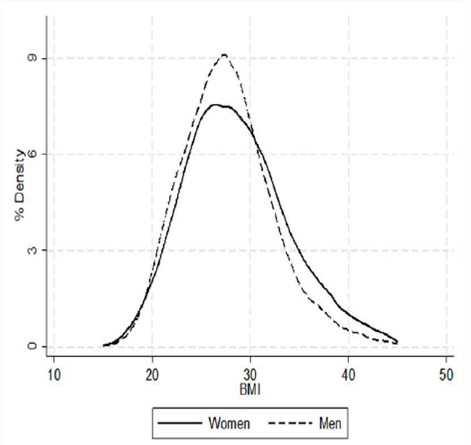
Note: Authors' calculation, using data from the ENSANUT 2012 (Barquera et al., 2013). Data restricted to individuals aged 20-60 years with a BMI from 15 to 45. The distribution was estimated using an Epanechnikov distribution with a bandwidth of 1.73. N= 30 452.
Figure 1 Body Mass Index Distribution
Figure 2 shows the normal (BMI < 25), overweight (25 < BMI < 30), and obese (BMI > 30) populations by sex, according to ENSANUT 2012. Over 40% of the men aged 20-60 are overweight, while 30% are obese. The corresponding proportions for women aged 20-60 are 36% and 38%. While 70% of the workforce is either overweight or obese, more men are overweight, while more women are obese.
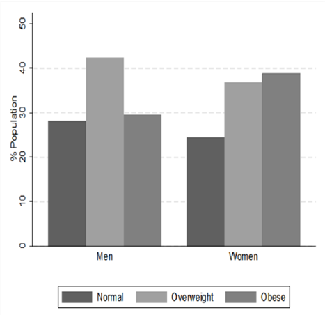
Note: Authors' calculation, using data from the ENSANUT 2012 (Barquera et al., 2013). Men and women aged 20-60 years. Severely obese is included with obese. N = 30 452.
Figure 2 Overweight and Obesity by Sex (%)
Table 1 presents descriptive statistics from the ENSANUT 2012. Column 1 presents information for the full sample, while column 2 is restricted to those who work. For the sample as a whole the aver-age age is 38, and more than half the individuals in the sample are married. The percentage of individuals who speak an indigenous lan-guage is 7.5%, while about 13% reported a recent illness. Men have an average of 9.1 years of schooling and women 8.6 years. As in many countries, the percentage of men working (70.4%) is higher than that of women (37.4%).
Table 1 Descriptive Statistics
| Full Sample (1) | Sample restricted to individuals who work (2) | |||
|---|---|---|---|---|
| Man | Women | Man | Women | |
| No. of observations | 12,724 | 17,728 | 8,931 | 6,067 |
| BMI | 27.7 | 28.6 | 27.8 | 28.8 |
| Standard deviation | 4.6 | 5.3 | 4.6 | 5.2 |
| BMI ≤ 25 (%) | 29.2 | 26.3 | 28.3 | 24.6 |
| Overweight (%) (25 < BMI ≤ 30) | 43.0 | 37.0 | 43.8 | 38.3 |
| Obese and severely obese (BMI > 30) (%) | 27.7 | 36.7 | 27.9 | 37.1 |
| Waist circumference (cm) | 96.6 | 91.9 | 94.7 | 91.9 |
| Standard deviation | 13.6 | 14.0 | 13.0 | 13.2 |
| Age(years) | 37.9 | 38.1 | 37.7 | 38.5 |
| Married (%) | 74.2 | 68.0 | 79.1 | 54.2 |
| Rural(%) | 24.4 | 24.2 | 23.4 | 15.6 |
| Speaks an indigenous language(%) | 7.3 | 7.5 | 6.6 | 5.2 |
| Health problems (%) | 13.2 | 16.6 | 12.8 | 18.4 |
| Years of schooling | 9.1 | 8.6 | 9.0 | 9.3 |
| At least a university degree(%) | 18.7 | 15.7 | 16.4 | 20.6 |
| Children 6-19 years old living in household (%) | 51.4 | 55.1 | 53.1 | 56.4 |
| Participation in the labor force (%) | 70.4 | 37.4 | 100.0 | 100.0 |
| Working hours per week | 48.7 | 37.7 | ||
| Monthly wage (pesos) | 5,999.2 | 4,643.5 | ||
| Hourly wage (pesos) | 28.4 | 28.4 | ||
| Full time employment (%) | 89.4 | 68.9 | ||
| Informal employment (%) | 62.6 | 67.2 | ||
Note: Authors' calculation, using data from the ENSANUT 2012 (Barquera et al., 2013). Column 1 presents data for all valid observations for the variables employed. Column 2 shows data only for workers in the sample restriction. Marriage includes cohabitation. Health problems in the 2 weeks before the survey. Wages given in constant Mexican pesos from January 2014. Full-time refers to at least 30 hours of work during the referenced week. Informal work is defined as work without access to social security. Waist circumference was observed for 97.5% of the sample in column 1 and 99.3% in column 2.
In the sample of individuals currently working (column 2), the average age is similar to that of the total sample. However, the pro-portion of married women is 13.8 percentage points less, and women's average years of schooling (9.3) is greater, while for men it is the same. The monthly labor income gap between men and women is approxi-mately 1,356 MXN (approximately 100 USD in January 2014).19 Men work an average of 10 hours more per week than women, but hourly wages are similar; the percentage of men working full time is nearly 90%, while for women the percentage is only 69%. The percentage of the working population that has no social protection is about 60% for both men and women.
Figures 3A and 3B present Lowess curves, the former showing the relationship between BMI and the percentage of individuals working, and the latter the relationship to real hourly wages of men and women. The proportion of men deciding to work is always higher than that of women. However, while the share of men deciding to work remains equal or diminishes slightly as the indicator of obesity is exceeded (BMI > 30), in women the effect is the opposite: a small increase when BMI exceeds 35. In the normal BMI range (20-25), women receive a higher hourly wage than men; however, as BMI increases to overweight and obesity levels, the gap narrows and turns in favor of men. Thus, men are rewarded for being overweight, whereas women are penalized with lower wages. A steady decline is observed in women's wages as BMI increases; the wages of a severely obese woman (BMI > 35) are about 20% less than those of a woman with a normal BMI. The wages of men with a BMI greater than 30 are approximately 15% less than those in the normal range.
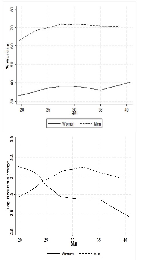
A. Percent of individuals working
Note: Authors' calculation, using data from the ENSANUT 2012 (Barquera et al., 2013). Data restricted to individuals with valid observations aged 20-60 years and BMI from 15 to 45. In panel A, N=30,452 (58.2% women); in panel B, N=14,998 (40.4% women). We define 20 quantiles of BMI by sex to generate a Lowess graph (using expansion weights in panel A and expansion weights multiplied by hours of work in panel B).
Figure 3 Labor Market Outcomes and BMI
Hourly wages for a woman with a BMI between 25 and 30 are up to 10% less than those of a man in the same range, while for an obese woman (BMI > 30) they are up to 15% less. This result is found not only in the ENSANUT 2012: there are similar differences in the Mexican Family Life Survey (MxFLS) for the period 2002-2012 (see Figures A1 and A2).
4. Methodology
Ideally, in order to show the causal effect of obesity on labor market outcomes, we would randomly place a group of individuals on different parts of the BMI scale and observe their labor market outcomes. However, as the ideal experiment is not available, we consider the use of instrumental variables (IV) to be the best way to approximate the situation. The application of instrumental variables has two foundations: the relevance and exclusion conditions of the instrument. The relevance condition requires the instrument to have a strong associa-tion with the variable that generates endogeneity: in our case, with BMI. The exclusion condition refers to independence between the instrument and the unobservable factors that also affect labor variables. In our case, these features can be expressed by the following equation:
We consider two scenarios: in the first, variable Y i is a dichoto-mous variable identifying whether the individual i works or not. The variable takes the value of 1 if the individual works at least one hour a week and 0 if not. In the second scenario, Y i represents the hourly wages received by individual i; they are expressed in logarithms and in constant January 2014 pesos. BMI is defined as weight in kilograms over the square of height in meters. Vector X expresses a set of covari-ates that seeks to capture characteristics of each individual and their household: age, years of schooling, indigenous language, marital status, current health status, and sociodemographic characteristics (rural area and socioeconomic region, of the seven defined by the Mexican institute of statistics). The IV assumptions thus require the instru-ment (z) to satisfy the relevance condition (Cov(BMI, z|X) = 0) and exclusion condition (Cov(z,e|X) = 0), controlling for characteristic X.
A key advantage of the ENSANUT is that it includes information on children living in the household, so there are height and weight data for children aged 6-19. We can thus restrict the IV sample to parents with children living in the same household and use the child's BMI as an instrument for that of the adult. As seen in Table 1 and Table 2, the sample of working individuals, 53.1% of men (4,350) and 56.4% of women (3,130), meets this restriction. 20 The challenge of this instrument is the exclusion restriction: if there is an omitted variable like stress, depression, or cognitive ability that determines the BMI of children and wages at the same time, the exclusion restriction is not valid.21 The ENSANUT does not include such measures, but we use the MxFLS data to estimate the relationship between BMI and labor market outcomes, controlling for depression and cognitive abilities, as described in Section 6.
Table 2 ENSANUT 2012, Descriptive Statistics (Restricted to households with a child aged 6-19 years)
| Full Sample (1) | Sample restricted to individual who work (2) | |||
| Man | Women | Man | Women | |
| No. of observations | 5,782 | 9,110 | 4,350 | 3,130 |
| BMI | 28.3 | 29.0 | 28.2 | 29.2 |
| Standard deviation | 4.4 | 5.1 | 4.3 | 5.0 |
| BMI ≤ 25 (%) | 22.1 | 22.1 | 22.4 | 19.2 |
| Overweight (25 < BMI ≤ 30) (%) | 47.1 | 39.2 | 47.2 | 41.8 |
| Waist circumference (cm) | 96.3 | 92.5 | 96.2 | 92.6 |
| Standard deviation | 12.2 | 13.3 | 12.0 | 12.5 |
| Age (years) | 41.5 | 38.6 | 40.9 | 39.2 |
| Married (%) | 97.2 | 80.4 | 97.3 | 65.1 |
| Rural (%) | 28.1 | 27.3 | 26.2 | 16.9 |
| Speaks an indigenous language (% | 9.7 | 9.2 | 7.8 | 6.4 |
| Health problems (%) | 12.8 | 16.4 | 12.1 | 18.4 |
| Years of schooling | 8.5 | 8.1 | 8.6 | 8.8 |
| At least a university degree (%) | 14.5 | 10.8 | 13.4 | 15.6 |
| Labor force participation (%) | 76.0 | 38.4 | 100.0 | 100.0 |
| Working hours per week | 49.5 | 36.6 | ||
| Monthly wage (pesos) | 6,047.3 | 4,476.5 | ||
| Hourly wage (pesos) | 28.2 | 28.3 | ||
| Full time employment (%) | 90.0 | 65.9 | ||
| Informal employment (%) | 62.3 | 71.7 | ||
Note: Authors' calculation, using data from the ENSANUT 2012 (Barquera et al., 2013). Column 1 presents data for all individuals with valid observations for the variables employed; column 2 shows data only for workers with valid observations. Marriage includes cohabitation. Health problems in the 2 weeks before the survey. Wages given in constant Mexican pesos from January 2014. Full-time refers to at least 30 hours of work during the referenced week. Informal work is defined as work without access to social security. Waist circumference is observed for 97.5% of the sample in column 1 and 99.4% in column 2.
5. Results
We present first the OLS results and then the IV results. Table 3 shows the OLS results of the effects of BMI on the dummy variable work (Yi) by sex, based on data from the ENSANUT 2012.22 Column 1 includes several variables as covariates: years of schooling (values from 0 to 16), age, age squared, and dummy variables for indigenous language, living in a rural area (less than 2,500 inhabitants), marital status, health condition, and socioeconomic region (of the seven defined by the Mexican statistics institute). Column 2 includes interactions between pairs of some of these variables: rural residence and years of schooling, and the age variables and years of schooling, in order to control for any additional bias correlated with these interactions.
Columns 3 and 4 include the restrictions in columns 1 and 2, respectively, and also reduce the sample size by eliminating those adults without a child aged 6-19 with a valid BMI. These data can be compared with the results from the IV sample. Finally, we grouped the results into four panels (A-D). Panel A estimates the effect of BMI on the probability of employment and Panel B estimates its effect on full-time employment (> 30 hours/week). Panel C estimates the effect of BMI on log of hourly wage and panel D the same effect for full-time workers.
The results presented in panel A are comparable for the two groups of covariates, for the whole and the IV sample. For the sample as a whole, the BMI is not related to the probability of employment for either men or women. Nor is there such a relationship for full-time workers (panel B). The coefficients in the IV sample are similar to those in the full sample. Restricting the sample to adults with children living in the household has a small negative effect on men (0.3 percentage points), but does not provide estimates for women different from those obtained using the full sample.
Panels C and D present the OLS estimates for the effect of BMI on the log of hourly wage. With the full sample, as shown in columns 1 and 2 of panel C, the effect of increasing BMI by one unit translates into a 0.8% reduction in women's hourly wage and a non-statistically significant reduction of 0.1% for men. Adding more control variables as interactions does not change the main estimates (columns 2 and 4). In sum, obesity only penalizes women's wages, not those of men. An increase in one standard deviation of BMI for women (5.3) results in a reduction of 4.2% in the hourly wage; that is, in one month, a woman would lose approximately 180 MXN (approximately 13 USD in January 2014).
These results are very close to those found for women in the United States, where a one standard deviation increase in BMI is associated with a reduction in hourly wages of approximately 3.5% (Pagan and Davila, 1997; Cawley, 2000; Han, Norton and Stearns, 2009; Han, Norton and Powell, 2011; Sabia and Rees, 2012). These effects are much greater, however than in European countries, where the average wage penalty is approximately 2% (Garcia and Quintana-Domeque, 2006). Interestingly, only in Sweden is a wage penalty observed for men, while in most other European countries the effect is positive but not significant (Lundborg, Nystedt and Rooth, 2014). Positive results for men are observed only in the United States and Belgium (3.5% and 2%, respectively; see studies by Cawley, Grabka and Lillard, 2005 and Garcia and Quintana-Domeque, 2006).
It is possible that the OLS coefficients are biased due to unobserved characteristics. We must, therefore, find a variable that is not related to unobservable factors that influence an individual's labor market outcomes. For this purpose, we can employ the BMI of children as an instrument for their parents' BMI. While it is feasible to corroborate the correlation between the instrument and individual BMIs, it is not possible to do so with the unobservable characteristics. In order to minimize this problem, we take advantage of a different database, one with a smaller sample than the ENSANUT, to validate our estimates controlling for depression and cognitive ability.
This specification, used by Cawley (2000) and Cawley, Grabka and Lillard (2005), is based on the premise that there is a genetic relationship between the BMI of children and that of their parents, and that the children's BMI does not affect the parents' labor market outcomes. Table 4 shows the IV results for the effect of BMI on labor market outcomes. The set of covariates are the same as in Table 3, including all interactions (columns 2 and 4); in addition, children's age is incorporated as a control for the variation in their ages. Finally, in order to analyze the degree of association between parents' and children's BMI, we incorporate an F test from the first stage. All of the F statistics in Table 4 are well above the minimum values suggested by Bound, Jaeger and Baker (1995) and Stock and Yogo (2005), demonstrating that childrens BMI is a useful instrumental variable.
Table 3 OLS Results
| (1) | (2) | (3) | (4) | |||||
| Men | Women | Men | Women | Men | Women | Men | Women | |
| A. Dep. Var. = 1 if Employed | ||||||||
|
BMI
N R2-Adj. |
-0.001 (0.001) 12,724 0.065 |
0.001 (0.001) 17,728 0.101 |
-0.001 (0.001) 12,724 0.074 |
0.001 (0.001) 17,728 0.107 |
-0.003* (0.002) 5,782 0.048 |
0.001 (0.001) 9,110 0.136 |
-0.004* (0.002) 5,782 0.055 |
0.001 (0.001) 9,110 0.140 |
| B. Dep. Var. = 1 if Full-Time Employee (FT) | ||||||||
|
BMI
N R2-Adj. |
-0.001 (0.001) 12,724 0.069 |
0.001 (0.001) 17,728 0.097 |
-0.001 (0.001) 12,724 0.077 |
0.001 (0.001) 17,728 0.101 |
-0.004* (0.002) 5,782 0.059 |
0.000 (0.001) 9,110 0.128 |
-0.005** (0.002) 5,782 0.064 |
0.000 (0.001) 9,110 0.128 |
| C. Dep. Var.: Log Hourly Wage | ||||||||
|
BMI
N R2-Adj. |
0.001 (0.002) 8,931 0.168 |
-0.008*** (0.003) 6,067 0.176 |
0.001 (0.002) 8,931 0.172 |
-0.008*** (0.003) 6,067 0.176 |
0.004 (0.003) 4,350 0.162 |
-0.008** (0.004) 3,130 0.156 |
0.004 (0.003) 4,350 0.167, |
-0.008** (0.004) 3,130 0.158 |
| D. Dep. Var.: Log Hourly Wage (FT) | ||||||||
|
BMI
N R2-Adj. |
0.000 0.002) 7,916 0.184 |
-0.007** (0.003) 4,196 0.232 |
0.000 (0.002) 7,916 0.189 |
-0.007*** (0.003) 4,196 0.234 |
0.003 (0.003) 3,862 0.183 |
-0.008* (0.004) 2,088 0.213 |
0.003 (0.003) 3,862 0.188 |
-0.008** (0.004) 2,088 0.222 |
Notes: Authors' calculations, using data from the ENSANUT 2012 (Barquera et al., 2013). Data restricted to individuals with valid observations for the variables employed. Robust standard errors in parentheses. Wage is given in Mexican pesos from January2014. ***p<0.01, **p<0.05, *p<0.1. Column 1 and 3 calculations include the following variables: rural, years of schooling, age, age squared, speaks an indigenous language, married, health problems, and a dummy variable for socioeconomic region. Column 2 and 4 calculations include interactions between the variables: rural - years of schooling, age - years of schooling, and age squared - years of schooling. Column 3 and 4 calculations restricted to individuals with children aged 6-19 with valid BMI.
Column 1 in Table 4 shows that a one-unit increase in BMI decreases men's probability of working by 0.3 percentage points (pp) and increases that of women by 1.2 pp. This significant result for women contrasts with the results obtained with OLS (See Table 3, Panel A, Column 4), which shows a positive, but not significant probability.
Table 4 IV Results
| Employed | Log Hourly Wage | |||
| Total | FT | Total | FT | |
| Women | ||||
| Children's BMI | 0.187*** | 0.187*** | 0.192*** | 0.205*** |
| (0.014) | (0.014) | (0.021) | (0.029) | |
| BMI | 0.012** | 0.010* | -0.032*** | -0.038*** |
| (0.006) | (0.005) | (0.018) | (0.014) | |
| N | 9,110 | 9,110 | 3,130 | 2,088 |
| R2-Adj. | 0.128 | 0.116 | 0.056 | 0.182 |
| F-weak id. | 189.5 | 189.5 | 84.64 | 51.71 |
| Men | ||||
| Children's BMI | 0.147*** | 0.147*** | 0.145*** | 0.138*** |
| (0.015) | (0.015) | (0.017) | (0.019) | |
| BMI | -0.003 | -0.002 | 0.016 | 0.019 |
| (0.009) | (0.009) | (0.017) | (0.018) | |
| N | 5,782 | 5,782 | 4,350 | 3,862 |
| R2-Adj. | 0.058 | 0.064 | 0.131 | 0.176 |
| F-weak id. | 99.1 | 99.1 | 75.59 | 53.07 |
Notes: Authors' calculations, using data from the ENSANUT 2012 (Barquera et al., 2013). Data restricted to individuals with valid observations for the variables employed. Wages given in Mexican pesos from January 2014. The average of children's BMI (age 6-19) is used as an instrument. Robust standard errors in parentheses. ***p<0.01, **p<0.05, *p<0.1. Variables included: rural, years of schooling, age, age squared, speaks an indigenous language, married, health problems, a dummy variable for socioeconomic region, and interactions between variables as follows: rural - years of schooling, age - years of schooling, and age squared - years of schooling.
However, we consider the OLS result could be biased as we mentioned before. Table 4 also includes results for full-time workers in Column 2, with the same sign and statistical significance as Column 1.
Columns 3 and 4 in Table 4 show the effect of BMI on hourly wages. A one-unit increase in BMI has significant negative effects on in women (3.2%); in men the effect is positive but not significant (1.6%).23 An increase of one standard deviation in a woman's BMI translates into a 16% reduction in hourly wages, or approximately 670 MXN monthly (50 USD in January 2014).24 Our estimates imply that an additional year of schooling translates into a 6.7% increase in wages.25 Hence, the impact on wages of a one standard deviation increase in womens BMI is equivalent to 2.5 fewer years of schooling. Column 4 shows that the results are similar across both the sample of all workers and the sample of those working full-time. The negative impact of BMI on wages is similar, though greater in absolute terms, than that found by Sabia and Rees (2012) for white women in the United States (13.1%), in which the BMI of a sibling was used as an instrument. Our estimate is also greater than that of Cawley (2004), in which a one standard deviation increase in a white woman's BMI in the United States is equivalent to 1.5 years of schooling (a negative effect on wages of 9%). In Europe, the same increase in a woman's BMI reduces her wages by 3-6% (Brunello and d'Hombres, 2007; Garcia and Quintana-Domeque, 2006). The impact of obesity in Mexico is much larger than in other countries, and the largest yet found, consistent with audit studies of discrimination in this country. Arceo-Gomez and Campos-Vazquez (2014) show that physical appearance has a direct effect on the probability of a woman receiving a response to an employment application, but not on men's. Future research could investigate whether differences in enforcement capacities across countries play a role in wage penalties due to physical appearance.
6. Robustness Checks
As previously mentioned, an unbiased estimation of the effect of obesity on wages and employment requires the fulfillment of certain conditions, including the relevance and exclusion conditions. Thus, we employ the BMI of children as an instrument independent of labor market outcomes to determine the effect of their parents' overweight or obesity on employment and wages. In other words, if we consider the BMI of children as a suitable instrument, it is possible to identify the effect of parents' obesity on the labor market. However, even if the instrument used complies with the relevant condition, it is not certain that it fulfills the exclusion condition, that is, that it is indeed independent of labor market outcomes. Table 5 thus presents addi-tional robustness tests for the wage results presented in the previous section.26 Angrist and Pischke (2008) recommend using limited information maximum likelihood ( LIML) instead of two-stage least squares (2 SLS) for estimation with weak instruments and small samples. In practice, however, because the F statistics are relatively large, both methods give similar results.
Table 5 Robustness Testing (Dep. Var.: Log Hourly Wage)
| (1) | (2) | (3) | (4) | (5) | (6) | |
| Women | ||||||
| BMI | -0.032*** | -0.027 | -0.033* | -0.030 | -0.032* | -0.033** |
| (0.018) | (0.018) | (0.017) | (0.019) | (0.018) | (0.014) | |
| N | 3,130 | 3,130 | 3,130 | 3,130 | 3,130 | 3,130 |
| F-weak id. | 84.64 | 78.75 | 86.29 | 69.21 | 85.18 | 23.08 |
| R2-Adj. | 0.056 | 0.064 | 0.055 | 0.059 | 0.056 | 0.133 |
| Hansen J stat. | 0.796 | |||||
| P-value | 0.672 | |||||
| Men | ||||||
| BMI | 0.016 | 0.013 | 0.007 | 0.026 | 0.015 | 0.012 |
| (0.017) | (0.017) | (0.017) | (0.018) | (0.017) | (0.012) | |
| N | 4,350 | 4,350 | 4,350 | 4,350 | 4,350 | 4,350 |
| F-weak id. | 75.59 | 76.18 | 74.52 | 67.61 | 76.23 | 51.68 |
| R2-Adj. | 0.131 | 0.133 | 0.134 | 0.119 | 0.133 | 0.164 |
| Hansen J stat. | 1.762 | |||||
| P-value | 0.4141 | |||||
Notes: Authors' calculations, using data from the ENSANUT 2012 (Barquera et al., 2013). Data restricted to individuals with valid observations for the variables employed. Robust standard errors in parentheses. Wages given in Mexican pesos from January 2014. ***p<0.01, **p<0.05, *p<0.1. The following variables are included: rural, years of schooling, age, age squared, speaks an indigenous language, married, health problems, a dummy variable for socioeconomic region, and interactions between variables as follows: rural - years of schooling, age - years of schooling, and age squared - years of schooling. Column 1 uses the average of children's BMI (age 6-19) as an instrument, column 2 the highest BMI of those children, column 3 the eldest child's BMI, and column 4 uses BMI of the youngest child. Column 5 uses the instrument of column 1 with the addition of the depression variable. In columns 1 to 5 we obtained the same results using LIML. Column 6 uses the instrument of column 1 and its second-and third-degree polynomials as instruments, estimated by LIML, following Dieterle and Snell (2014).
Table 5, column 1, shows the same regression as Table 4. This estimate is obtained using the average BMI of individuals' own children as an instrument. We test whether this result is driven by the BMI of one child in particular. A priori, we would expect that if the instrument is valid, i.e., that the BMI of any of the children is related to the BMI of their parents but without unobservable factors, there should be no difference with respect to which child's BMI is used. Columns 2, 3, and 4 use, respectively, the highest BMI among them, the BMI of the eldest child aged 6-19, and the BMI of the youngest of the group as instruments.
The negative effects remain very close to those of the main regression (2.7%, 3.3%, and 3%, respectively). In other words, a one-unit increase in the BMI, was associated with a 2.7%, 3.3% and 3% decline in hourly wage for women. In all cases, F tests allow us to reject the null hypothesis of weak instruments. However, the result is only significant when we use the BMI of the eldest child.27
Another possible explanation for the effect of obesity on wages can be low self-esteem or depression. People with low self-esteem or depression may be careless of their health, appearance, and effort on the job, which may affect their wages. If this assertion is correct, omitting this indicator in the estimation would bias the results. However, the incorporation of depression as an explanatory variable in the regression is not a simple task, as depression may also be an endogenous result of obesity and lack of success in the labor market. Column 5 incorporates a standardized measure of depression (this variable was built on seven questions in the ENSANUT regarding such symptoms as sadness, depression, lack of concentration, and insom-nia). The results are similar to the main regression, where the hourly wage penalty for a one-unit increase in the BMI is concentrated mainly among women (-3.2%).
Finally, Dieterle and Snell (2014) have proposed using the in-strument along with its higher-order polynomials in the estimation. Given no heterogeneous treatment effects, using a linear or a polyno-mial specification of the instrumental variable in the first stage should not affect the main estimate in the second stage if the instruments are valid. The exogeneity condition implies that the squares or cubes of the instrument should also not be correlated with the unobserved components (term e in Equation 1). Column 6 uses this method on the instrument in Column 1 and incorporates its second- and third-order polynomials; it also includes the p-value of the overidentification test. The results are close to those of the main regression, and we cannot reject the null hypothesis that the additional instruments are valid.
Table 6 shows further evidence of robustness by using the three rounds of the MxFLS on the same regressions estimated using the ENSANUT.28 As the MxFLS sample is smaller, standard errors increase substantially.29 Column 1 uses the same instrument as column 1 of Table 4 (average BMI of the children aged 6-19). As with the analysis using the ENSANUT, for men the estimates are not statistically signif-icant. In the case of women, even though the effect is not significant, the result is very close to that found in the first analysis (2.1%).
Table 6 Robustness Results Using the Mexican Family Life Survey (Dep. Var.: Log Hourly Wage)
| (1) | (2) | (3) | (4) | (5) | |
| Women | |||||
| BMI | -0.021 | -0.016 | -0.016 | 0.008 | -0.020 |
| (0.020) | (0.019) | (0.019) | (0.013) | (0.019) | |
| N | 2,693 | 2,693 | 2,693 | 875 | 2,693 |
| F-weak id. | 53.69 | 62.32 | 62.67 | 109.2 | 54.42 |
| R2-Adj. | 0.208 | 0.207 | 0.211 | 0.157 | 0.227 |
| Men | |||||
| BMI | 0.008 | 0.004 | 0.010 | 0.011 | 0.009 |
| (0.014) | (0.017) | (0.017) | (0.008) | (0.014) | |
| N | 5,265 | 5,265 | 5,265 | 1,533 | 5,265 |
| F-weak id. | 150.5 | 108.1 | 102.6 | 712.2 | 150.6 |
| R2-Adj. | 0.211 | 0.201 | 0.209 | 0.169 | 0.214 |
Notes: Authors' calculations, using data from the MxFLS, rounds 1-3. Data restricted to individuals with valid observations for the variables employed. Robust standard errors in parentheses. Wages given in Mexican pesos from January 2014. ***p<0.01, **p<0.05, *p<0.1. Column 1 includes the following variables: rural, years of schooling, age, age squared, speaks an indigenous language, married, health problems, dummy variables for socioeconomic region and year of the survey, and interactions between variables as follows: rural - years of schooling, age - years of schooling, and age squared - years of schooling. Column 1 here uses the same instrument as column 1 in Table 5. Column 2 uses the highest BMI among children aged 6-19 as an instru-ment and the same variables as column 1, without the interactions. Column 3 uses the highest BMI among children aged 6-19 and all the variables from column 1, column 4 the BMI of the individual in the first round and all the variables of column 1, and column 5 uses the instrument of column 1 with the addition of the variables depression and cognitive ability. In columns 1 to 5 we obtain the same results using LIML.
Columns 2 and 3 are analogous to the analyses using the EN-SANUT. Column 2 uses the highest BMI among children aged 6-19 as instrumental variable and column 3 the BMI of the eldest child. The results are similar but noisier and no longer statistically significant.
Taking advantage of the longitudinal nature of the MxFLS, column 4 uses as an instrument the individual BMI from round 1 for the same individual's results in round 3, following Cawley (2000). The results are not statistically significant. However, this instrument may be in-appropriate if we expect that an early BMI measure is related to a current labor market decision.
Column 5 uses the same instrument as column 1 (average BMI of children aged 6-19) but adds the measures of depression and cognitive ability of the individual as right-hand-side variables. 30 Using these variables we seek to control for individual characteristics, which can have effects on both obesity and wages. Thus, it is possible that depression has a direct impact on people's eating patterns and at the same time a relationship with wages. A similar argument could be made with cognitive skills. However, it should be mentioned that, as in Table 5, column 4, the depression measure must be incorporated with caution, as it may be endogenous to the model. The results indicate that the effects of BMI in men are positive and not significant (0.9%), and very close to those found in column 1. The negative results for women remain the same (2%) as those in the regression with data from the ENSANUT and the additional robustness tests.
Averett (2014) notes that waist circumference is a measure of central obesity. It has the key advantage over BMI that it is a stronger predictor of mortality and morbidity. In addition, it is a good measure of visible fatness, which may lead to discrimination. The ENSANUT includes exact measurement of waist circumference: the average for women is 91.9 cm, with a standard deviation of 13.2 (Table 1). Table 7 is analogous to Table 6 but uses the log of waist circumference in-stead of BMI on the log of hourly wages.31 Column 1 uses the log of children's waist circumference as an instrument. As in previous tables, the only statistically significant effects are for women. Columns 2-5 use the largest waist circumference among the children, the waist circumference of the eldest child, the main instrument (column 1) with the depression variable as a control, and the main instrument with its second- and third-degree polynomials.32 The results are con-sistent with those shown in Table 5. There is a negative effect of BMI or waist circumference on women's wages but not on men's wages. An increase of one standard deviation in waist circumference reduces women's wages by 24%, which is larger than the effect of a one standard deviation increase in BMI.
Table 7 Robustness Testing Using Waist Circumference (Dep. Var.: Log Hourly Wage)
| (1) | (2) | (3) | (4) | (5) | |
| Women | |||||
| Log. waist circumference | -1.717** | -1.754** | -1.620** | -1.688** | -1.531** |
| (0.801) | (0.810) | (0.788) | (0.805) | (0.650) | |
| N | 2,620 | 2,620 | 2,620 | 2,620 | 2,620 |
| F-weak id. | 20.94 | 21.51 | 19.23 | 20.65 | 29.29 |
| R2-Adj. | 0.092 | 0.089 | 0.099 | 0.095 | 0.106 |
| Hansen J stat. | 1.105 | ||||
| P-value | 0.576 | ||||
| Men | |||||
| Log. waist circumference | -0.021 | 0.086 | 0.036 | -0.069 | 0.607 |
| (1.019) | (1.050) | (1.006) | (1.012) | (0.578) | |
| N | 3,500 | 3,500 | 3,500 | 3,500 | 3,500 |
| F-weak id. | 19.14 | 18.03 | 19.45 | 19.75 | 34.45 |
| R2-Adj. | 0.164 | 0.165 | 0.164 | 0.163 | 0.161 |
| Hansen J stat. | 0.630 | ||||
| P-value | 0.730 | ||||
Notes: Authors' calculations, using data from the ENSANUT 2012 (Barquera et al., 2013). Data restricted to individuals with valid observations for the variables employed. Robust standard errors in parentheses. Wage is given in Mexican pesos from January 2014. ***p<0.01, **p<0.05, *p<0.1. The following variables are included: rural, years of schooling, age, age squared, speaks an indigenous language, married, health problems, a dummy variable for socioeconomic region, and interactions between the variables as follows: rural - years of schooling, age - years of schooling, and age squared - years of schooling. Column 1 uses the log of the average of children's waist circumference as an instrument, column 2 the log of the largest waist circumference among children, column 3 the log of the eldest child's waist circumference, column 4 the instrument from column 1 with the addition of the depression variable, and column 5 the instrument of column 1 with its second- and third-degree polynomials, estimated by LIML, following Dieterle and Snell (2014). Average log waist circumference is 4.5 for both men and women. Standard deviation is 0.13 for men and 0.14 for women.
Table 8 repeats the analysis in Table 5 but incorporates as explanatory variables, the effects of age and sex of the children used as instruments.33 The BMI of children and teenagers increases naturally during those stages of life; the inclusion of these variables provides a control for this effect (Onis et al., 2007). In the case of hourly wages, the negative effect for women remains, but is slightly greater. In the case of men, the results are statistically significant only when we use the average BMI and the BMI of the youngest child (columns 1 and 4).
Table 8 Robustness Testing (Dep. Var.: Log Hourly Wage)
| (1) | (2) | (3) | (4) | (5) | (6) | |
| Women | ||||||
| BMI | -0.037*** | -0.032** | -0.033** | -0.047*** | -0.037*** | -0.031** |
| (0.013) | (0.013) | (0.014) | (0.014) | (0.013) | (0.012) | |
| N | 3,018 | 3,018 | 3,018 | 3,018 | 3,018 | 3,018 |
| F-weak id. | 77.64 | 87.13 | 86.00 | 67.74 | 77.61 | 35.41 |
| R2-Adj. | 0.129 | 0.140 | 0.140 | 0.103 | 0.131 | 0.141 |
| Hansen J stat. | 1.915 | |||||
| P-value | 0.384 | |||||
| Men | ||||||
| BMI | 0.019* | 0.018 | 0.016 | 0.026** | 0.018 | 0.015 |
| (0.011) | (0.011) | (0.012) | (0.011) | (0.011) | (0.011) | |
| N | 4,207 | 4,207 | 4,207 | 4,207 | 4,207 | 4,207 |
| F-weak id. | 142.80 | 87.07 | 142.20 | 63.80 | 144.30 | 58.01 |
| R2-Adj. | 0.158 | 0.161 | 0.164 | 0.146 | 0.160 | 0.162 |
| Hansen J stat. | 3.292 | |||||
| P-value | 0.193 | |||||
Notes: Authors' calculations, using data from the ENSANUT 2012 (Barquera et al., 2013). Data restricted to individuals with valid observations for the variables employed. Robust standard errors in parentheses. Wages given in Mexican pesos from January 2014. ***p<0.01, **p<0.05, *p<0.1. The following variables are included: rural, years of schooling, age, age squared, speaks an indigenous language, married, health problems, a dummy variable for socioeconomic region, and interactions between variables as follows: rural - years of schooling, age - years of schooling, and age squared - years of schooling. Column 1 uses the average of children's BMI (age 6-19) as an instrument, column 2 the highest BMI of those children, column 3 the eldest child's BMI, and column 4 the youngest child's. Column 5 uses the instrument of column 1 with the addition of the depression variable. In columns 1 to 5 we obtained the same results using LIML. Column 6 uses the instrument of column 1 and its second- and third-degree polynomials as instruments, estimated by LIML, following Dieterle and Snell (2014).
Finally, Table 9 uses as an instrument a normalized measure of the BMI of children (z-scores) in order to capture the effect of age and sex of these variables.34 Following Onis et al. (2007), we build z-scores for the BMI of the children and limit the sample to the range of 4-5, following Freedman et al. (2015). The results show that in the case of hourly wage, the negative effect remains for women, but is not significant for men, except in columns 4 and 6, where we use the BMI of the youngest child.
Table 9 Robustness Testing (Dep. Var.: Log Hourly Wage)
| (1) | (2) | (3) | (4) | (5) | (6) | |
| Women | ||||||
| BMI | -0.031** | -0.028* | -0.030** | -0.033** | -0.035** | -0.032** |
| (0.015) | (0.015) | (0.015) | (0.016) | (0.014) | (0.013) | |
| N | 3,006 | 3,006 | 3,006 | 3,006 | 3,006 | 3,006 |
| F-weak id. | 137.70 | 136.60 | 139.90 | 114.40 | 73.61 | 34.26 |
| R2-Adj. | 0.065 | 0.069 | 0.067 | 0.062 | 0.139 | 0.138 |
| Hansen J stat. | 0.635 | |||||
| P-value | 0.728 | |||||
| Men | ||||||
| BMI | 0.017 | 0.010 | 0.014 | 0.019* | 0.017 | 0.018* |
| (0.011) | (0.011) | (0.011) | (0.011) | (0.011) | (0.011) | |
| N | 4,199 | 4,199 | 4,199 | 4,199 | 4,199 | 4,199 |
| F-weak id. | 220.00 | 212.70 | 192.50 | 194.90 | 189.30 | 68.50 |
| R2-Adj. | 0.133 | 0.137 | 0.135 | 0.131 | 0.164 | 0.159 |
| Hansen J stat. | 0.471 | |||||
| P-value | 0.790 | |||||
Notes: Authors' calculations, using data from the ENSANUT 2012 (Barquera et al., 2013). Data restricted to individuals with valid observations for the variables employed. BMI of the instrument in z-scores. Robust standard errors in parentheses. Wage is given in Mexican pesos from January 2014. ***p<0.01, **p<0.05, *p<0.1. The following variables are included: rural, years of schooling, age, age squared, speaks an indigenous language, married, health problems, a dummy variable for socioeconomic region, and interactions between the variables as follows: rural - years of schooling, age - years of schooling, and age squared - years of schooling. Column 1 uses the average of children's BMI (age 6-19) as an instrument, column 2 the highest BMI of those children, column 3 the eldest child's BMI, and column 4 the youngest child's. Column 5 uses the instrument of column 1 with the addition of the depression variable. In columns 1 to 5 we obtained the same results using LIML. Column 6 uses the instrument of column 1 and its second- and third-degree polynomials as instruments, estimated by LIML, following Dieterle and Snell (2014).
7. Conclusion
Mexico has the second highest rate of obesity in the world (32.4%), exceeded only by the United States, and it is the country with the highest obesity rate for women (37.5%). Although there are many studies analyzing the relationship between obesity and labor market outcomes, an examination of Mexico is of particular importance for three reasons. First, Mexico offers a large variation in body mass index, with 27.5% of individuals in the normal range, 39.6% overweight, and 32.8% obese. Second, Mexico has a health survey including exact measurements of height, weight, and waist circumference, along with labor market outcomes. Third, previous estimates are mainly for developed countries with effective institutions for sanctioning discrimination.
We find two sets of important results. First, BMI has no relationship with men's decision to work whereas, it has a small and positive effect on women. Second, increased BMI affects women's wages but not that of men. Using an instrumental variable approach, we find that an increase in the BMI of one standard deviation lowers women's wages by 16%. This effect is substantial, equivalent to a decrease of 2.5 years in schooling. The effects we find are similar to, but greater than, those found for white women in the United States (Cawley, 2004; Sabia and Rees, 2012), and much larger than estimates for European countries (Brunello and d'Hombres, 2007; Garcia and Quintana-Domeque, 2006). Finally, our results are highly robust to the sample used, as well as with control variables for depression and cognitive skills. A key question for future research is whether differences across countries in the extent of wage penalties due to obesity are driven by institutional capacities to prevent discrimination.

