nueva página del texto (beta)
 Inglés (pdf)
 Artículo en XML
 Referencias del artículo
 Enviar artículo por email
 Citado por SciELO
  Similares en
SciELO
Similares en
SciELO 
 Permalink
1. Introduction
The intergenerational mobility (IGM) model is concerned with the relationship between the socio-economic status of parents and the socio-economic outcomes of their children as adults (Blanden, 2013). According to Torche (2013), this socioeconomic standing is captured by different measures, but the most common ones are individual earnings, family income, social class, and employment status. In particular, employment status provides a good proxy for long-term economic standing because it remains relatively stable over the individual’s employment career, so that a single measure can yield adequate long-run information (Fox, Torche and Waldfogel, 2016).
Recent evidence shows that family background has a significant impact on the sector of employment of their children. In particular, evidence shows that children of self-employed or informal workers are significantly more likely to be self-employed or work in the informal sector (Hout and Rosen, 2000; Colombier and Masclet, 2008; Pasquier-Doumer, 2012). Some researchers argue that informal employment is the result of an optimal choice. As such, informal workers choose informality because they expect higher welfare there than in the formal sector (Maloney and Ribeiro, 1999; Maloney, 2004; Packard, 2007).
Understanding the relationship between parents and sons’ work choices is essential for assessing the opportunities for social mobility. In fact, the intergenerational transmission of self-employed or informal sector status is frequently connected with higher expected earnings (Fairlie and Robb, 2006; Colombier and Masclet, 2008). Although there is no consensus on the voluntary nature of working in the informal sector, evidence points to a strong intergenerational transmission of employment status (Pasquier-Doumer, 2012).
In Mexico, the way that social mobility has been measured depends on the specific aspects of social mobility being investigated, as well as on the available data. Until now, research regarding intergenerational transmissions of formal/informal employment sector has focused only on sons and parents living in the same household (Valero and Tijerina, 2003; Castillo and Vela, 2013), mainly because there is no adequate data from longitudinal surveys.
This paper uses a retrospective data collection from the ESRU survey of social mobility in Mexico, EMOVI 2011, CEEY (2011), which allows us to explore how a worker’s formal/informal employment sector is affected by the employment sector of her/his parents. Our study differs from previous studies in Mexico in two ways: (1) the micro-econometric framework is derived from a structural model with expected wages explicitly determining employment sector decisions, (2) selectivity bias is controlled for using Lee’s (1982) procedure. The outline of the paper is as follows. Section 2 briefly examines some of the associated literature. Section 3 introduces the model and discusses its identification. Section 4 highlights a few features from the data and presents results. Section 5 concludes.
2. Literature review
A large number of economists suggest that labor markets are segmented. Lewis (1954) and Harris and Todaro (1970) propose that developing countries are characterized by a dual labor market, consisting of a modern formal sector and a large, less-efficient, informal sector. These two sectors seem to be operating different labor markets. One offers better paid and more attractive jobs, while the secondary, informal sector, is characterized by rather low pay, unqualified workers, and short term jobs (Eichhorst and Kendzia, 2014). Secondary sector jobs are characterized by low (or even zero) marginal productivity which justifies in part the low wages paid. Hence, informal employment appears as a constrained choice (Rauch, 1991; Magnac, 1991; Pasquier-Doumer, 2012; Mboutchouang, Kenneck and Mbenga, 2013).
However, recent literature for some countries have proposed a different perspective: informal sector is the result of an optimal choice where individuals expect a higher welfare there than they would obtain in the formal sector (Maloney and Ribeiro, 1999; Packard, 2007). This literature views the informal sector as an active and voluntary entrepreneurial small-firm sector, where individuals choose to work because they expect a greater welfare than if they were wage-earners or formal-sector entrepreneurs (Maloney, 2004). In this sense, a proportion of informal employment may reflect an efficient allocation of labor (PasquierDoumer, 2012).
In addition, the possibility that both types of informal employment exist simultaneously has also been proposed (Fields, 1990; Perry et al., 2007). Alcaraz, Chiquiar and Salcedo (2015) estimate that 10 to 20 percent of informal workers in Mexico are voluntarily self-selected into the informal sector.
Although there is no consensus on the -at least partially- voluntary nature of informal employment, some facts lead to certain reflections on individuals self-selecting to work in the informal sector and on the intergenerational transmission of informal entrepreneurship status (De Paul, Massil, and Modeste, 2013). In this sense, some authors have suggested that segmented labor markets must be characterized by low mobility between formal and informal jobs must be observed; while self-selected informal employment markets should have the opposite characteristic (Fiess, Fugazza and Maloney, 2010).
In addition, in the economic literature, the intergenerational transmission of formal or informal employment is sometimes connected with higher expected earnings, which is consistent with the non-segmented labor market view (Colombier and Masclet, 2008; Fairlie and Robb, 2006). In Mexico, nearly 60 percent of workers have informal jobs (ILO, 2014), operating small establishments with low capital labor ratios (Leal-Ordoñez, 2014). Moreno (2007) estimates the average conditional difference between both sectors using Mincer equations. After controlling for selectivity among workers, he finds that workers with higher levels of education earn more in the formal sector; and workers with high school or less receive higher wages in the informal sector. These results are similar for women with basic and secondary schooling.
With regard to the choice of becoming employed in the formal or in the informal sector in Mexico, Duval and Smith (2011) modify Dickens and Lang (1985) methodology to allow for voluntary and involuntary informal workers. The authors find that free social protection programs (such as Mexico’s “Seguro Popular”) reduce the incentives for employment in formal sector jobs. In addition, Huesca and Padilla (2012) use a counterfactual technique to estimate wages if workers were employed in both sectors. The authors estimate that workers with higher schooling are more likely to work in the formal sector and women with lower education levels have a higher probability of working in the informal sector. However, he found that these probabilities change with age.1
Few studies have addressed individual wages from an intergenerational approach in Mexico. In an early paper, Valero and Tijerina (2003) estimate Mincer equations for workers controlling for their parents’ characteristics, including wages, schooling, and employee status. The authors find that sons of employers and self-employed parents have higher wages than sons of employees. The authors suggest that this is caused by the transmission of skills, training, and entrepreneurial abilities.
As evidence for the intergenerational transmission of sectors of employment in Mexico, Castillo and Vela (2013) use a probit model to estimate the probability that sons choose the same sector than their parents. Their results suggest that the social-domestic context has an influence in their labor decisions, suggesting that self-employed parents transmit informal human capital to their sons during childhood.
However, the main limitation of these last two studies is that they only obtain information for sons and parents living in the same household at the moment of the interview. This fact not only reduces the sample size considerably (by almost 90%) but also may introduce important biases given that sons may choose to stay at parent’s home for non-random reasons.
This research overcomes this problem using EMOVI 2011. Unlike previous surveys in Mexico, EMOVI 2011 provides retrospective data that allows us to connect current respondents’ information and their comparable retrospective data from parent’s and family conditions when the interviewee was 14 years old. This allows us to recover data for both cohabiting and non-cohabiting children.
3. Empirical strategy
3.1. Identification
A key issue for examining the determinants of labor payments is the preferences of workers. In a narrow sense, we might be interested in asking why a worker chooses to work in a particular sector. The model used here is based on a binary representation of the sector of employment decision. It assumes that there are two employment options available to each individual: formal and informal sectors. In addition, two important features should be considered. First, the informal sector regime is associated with more flexibility and independence than the formal sector. And second, each sector has different working conditions and different market institutions.
Similar to Rees and Shan (1986), we assume that the sector of employment and wages are determined simultaneously. This requires a 3SLS estimation procedure. In the first stage, we estimate a reduced-form probit model of sector of employment decision. This is used to construct a sample selection correction term. In the second stage, we estimate an OLS standard Mincer equation to estimate the earnings function. This is used to compare the differences in wages between both sectors, and to correct the bias in sample selection. And finally, in the third stage, the differences in wages are used to estimate a probit model of the decision to be employed in the formal or informal sector.2
Assuming that workers choose between working in the formal or informal sector, we
specify a linear utility function, Uk that represents the utility
derived by individual i working in either sector: Individual i decides to work
in the formal sector if
Equation (1) below defines the probability that individual i works in the formal sector as a function of his own earnings differences (log Yformal − log Yinformal ) and other worker characteristics (Xi) as follows:
Equation (1) can be estimated as a probit model. However, a worker’s earnings are only observed for the sector in which the worker is actually working. In order to run Equation (1) we need an estimate of the potential earnings in the other sector for each worker. Since worker’s earnings in a particular sector may depend on the potentially self-selected characteristics of the workers, the Lee (1982) two-stage procedure must be used to construct such predicted earnings (Koumenta, 2011).
To address this issue, we estimate two Mincer’s (1974) semi-logarithmic wage equations, one for the formal workers (log Yformal) and other for the informal workers (log Yinformal ). As independent variables, we use worker characteristics (Xi) and their parent’s characteristics (Zi).
Mincer’s semi-logarithmic wage equations are defined as follows:
The model is identified by the exclusion in Equations (2) and (3) of at least one element of Xi in Equation (1). Equation (1) can then be estimated using the standard maximum likelihood procedure. Estimating income Equations (2) and (3) by Ordinary Least Square (OLS) might be inappropriate because it fails to reflect the possibility of self-selection in the decision to choose a sector of employment: workers might have some unobserved characteristics that affect their income generating capabilities in each sector.
To deal with possible self-selection bias, Lee’s (1982) methodology recommends substituting income Equations (2) and (3) into (1) and obtaining the reduced form of the sector of employment decision Equation (1).
Assuming that the error term (
The selectivity correction variables, H 1i and H 0i, measure the truncation effect associated with sample selectivity (see, e.g. Lee, 1982) and are included in the two income Equations (2) and (3) to control for self-selection as follows:
Thus, (
Finally, the OLS predicted values of earnings for individuals in both formal ln(
4. Data
4.1. Informal employment definition
Measuring the size of the informal economy and the incidence of informal employment is a difficult task. Also, different definitions have been put forward to make the concept operational. The appropriate methodology for the statistical measurement of informal employment depends on the users’ requirements, measurement objectives, and the organization of the information.
Several definitions of the dividing line between formal and informal employment exist. For statistical proposes, the International Labor Organization (ILO) in The Fifteen International Conference of Labor Statistician Characterized (15th ICLS resolution) uses the following criteria: informal employment “...encompasess a person in employment who, by law or in practice, are not subject to national labor legislation and income tax or entitled to social protection and employment benefits...” (ILO, 2013: 4).6
Following one of the above criteria, in this paper, informal employment is defined as employees without access to public or private health insurance. This criterion is especially useful in countries where the registration of workers entails the registration of the enterprises employing them with social security institutions (most notably, in Mexico, through its social security agencies, such as IMSS and ISSSTE).
Although the employment relationships of workers in informal employment are heterogeneous, they share a basic vulnerability, which is that they need to be self-supporting and to rely on informal arrangements with respect to social protection needs.7,8
4.2. Social mobility survey
The individual information used in this study is taken from the 2011 ESRU Survey of Social Mobility in Mexico, EMOVI 2011, that covers both rural and urban areas. EMOVI provides information about individuals between 25 and 64 years old (both household heads and non-household heads) from 11 001 households over two generations. This survey tracks the socioeconomic variables of a given household; each household member is asked detailed questions about age, gender, marital status, educational level, labor market participation, working hours, employment status and other work-related variables, as well as household size and other family features. In addition, a retrospective survey is applied, with each adult member of the household asked detailed information about characteristics of their parents and family conditions when the interviewee was 14 years old. Such information includes parents’ labor market participation and parents’ working conditions.9,10
4.3. Sample and descriptive statistics
Since our goal is to study the interaction between sons and parents’ sector of employment, we define our estimation sample according to the criteria that emphasizes coverage by the social security system. In the EMOVI 2011 survey, informal work regime is identified by the question: As part of this job do you receive health care benefits? This question is applicable for sons and their parents.
As in many labor research projects, we exclude female workers to prevent the results from being affected by sample selection bias, due to women’s low rates of labor participation in Mexico (Caamal, 2007; Campos and Velez, 2014). This restriction is justified by the aim of forming a relatively homogeneous sample of employment occupations and wages.
We restrict the sample to full-time male workers (defined for our purpose as those who only have one job and work 30 or more hours per week) who provide information on their earnings and sector of employment. Part-time workers usually have more unstable work behavior, affecting the precision and significance of the estimators.11 We keep only those who report being wage or salaried workers and exclude all others, because salaried workers are those to whom health care obligations apply. In the case of earnings, we exclude observations with values smaller than the 1st percentile or larger than the 99th percentile. This cutoff point is of course arbitrary, but it is frequently used in related studies.12
The final sample consists of 2 851 full-time male workers between 25 and 64 years old. Table A1 in the Appendix contains a summary of the statistics of the sample, including maximum, minimum, mean and standard deviation of each variable.
As a starting point, Table 1 reports the intergenerational mobility regime. Each row of the table shows the sector of employment of the fathers while columns indicate the sector of employment of the sons. It shows that 62 percent of respondents work in the same sector as their parents: 39 percent of formal-sector workers reported that their parents also worked in the formal sector, and 75 percent of informal-sector workers report that their parents were also employed in the informal sector. Clearly, the percentage of sons that stay in the same sector as their parents is considerably larger in the informal sector.
Table 1 Intergenerational mobility between sectors of employment
| Father’s employment sector | Son’s employment sector | Total | |
|---|---|---|---|
| Formal worker | Informal worker | ||
| Formal worker | 403 | 628 | 1 031 |
| (%) | 39 | 61 | 100 |
| Informal worker | 452 | 1 368 | 1 820 |
| (%) | 25 | 75 | 100 |
| Total | 855 | 1 996 | 2 851 |
| (%) | 30 | 70 | 100 |
Source: Author’s calculation based on 2011 EMOVI.
Table 2 provides descriptive statistics by employment status. Although there are significant differences between individuals working in the formal and informal sector in all respects, the informality wage penalty cannot be calculated simply looking at differences in the logarithm of the hourly wage. Regression analysis is required to find the ceteris paribus effect of the sector of employment upon earnings.
Table 2 Descriptive statistics by sector of employment
| Variable | Formal workers | Informal workers | Mean difference | ||
|---|---|---|---|---|---|
| (Obs = 855) | (Obs = 1 996) | ||||
| Mean | SD | Mean | SD | ||
| Log hourly wage | 3.244 | 0.655 | 2.876 | 0.749 | 0.368*** |
| Age | 35.724 | 9.852 | 37.511 | 11.667 | -1.787*** |
| Labor experience | 18.957 | 11.156 | 23.177 | 13.572 | -4.220*** |
| Less than primary | 0.053 | 0.223 | 0.161 | 0.368 | -0.109*** |
| Primary completed | 0.143 | 0.35 | 0.24 | 0.427 | -0.097*** |
| Secondary completed | 0.636 | 0.481 | 0.556 | 0.497 | 0.080*** |
| University completed | 0.168 | 0.374 | 0.043 | 0.202 | 0.126*** |
| Father’s years of schooling | 5.172 | 4.428 | 3.532 | 3.905 | 1.640*** |
| Mother’s years of schooling | 4.988 | 4.074 | 3.472 | 3.762 | 1.516*** |
Note: * p< 0.1, ** p<0.05, *** p<0.01. Source: Author’s calculation based on 2011 EMOVI.
Our data shows that the standard deviation in the logarithm of the informal-sector hourly wage exceeds the standard deviation of the formal sector wage, and it seems plausible that informal sector incomes may in fact be more vulnerable to shocks than formal sector incomes. In addition, significant differences are observed in age, potential labor experience, and schooling levels. Also, we observed that formal workers were more likely to have parents with more years of schooling.13
5. Results
5.1. Correcting for the self-selection bias
Following the empirical strategy defined in section 3, the first step in
correcting for self-selection bias is to estimate the probability of working in
the formal sector as in Equation
(4), including as independent variables: marital status, labor
experience, labor experience squared, parents’ employment sector, community
size, and dummies for region. The estimated coefficients of these variables are
reported in Table A2 in the Appendix. With the fitted values of Equation (4) at hand, we compute
both inverse Mill’s ratios
The formal workers wage Equation (5) and informal workers wage Equation (6) also include, as regressors, the selection coefficient or inverse Mills ratio, H 1 and H 0, respectively. The exercise is performed for the entire sample and for two groups of workers according to their level of schooling: middle school or less and high school or more. Estimated coefficients are displayed in Table 3. The coefficients in the wage equations report the estimates for selectivity correction terms H 1 and H 0. In both cases they are statistically significant.14
Table 3 Coefficients of selectivity variables in wage regressions
| Equation (5) | Equation (6) | |||||
|---|---|---|---|---|---|---|
| Formal wage equation | Formal wage equation | |||||
| All sample | Less- skilled workers | More- skilled workers | All sample | Less- skilled workers | More- skilled workers | |
| Married | -.088 | -.021 | -.086 | -.041 | -.031 | -.079 |
| (.050) | (.066) | (.054) | (.038) | (.046) | (.049) | |
| Age | .012*** | .003 | .013*** | .005** | .005* | .010*** |
| (.003) | (.004) | (.003) | (.002) | (.002) | (.003) | |
| H1 | .563*** | .144 | .491*** | |||
| (.102) | (.146) | (.116) | ||||
| HO | -1.092*** | -1.029*** | -1.017*** | |||
| (.120) | (.172) | (.143) | ||||
| Const. | 3.628*** | 3.276*** | 3.612*** | 2.350*** | 2.303*** | 2.297*** |
| (.148) | (.196) | (.173) | (.119) | (.152) | (.147) | |
| Obs. | 852 | 403 | 686 | 1 985 | 1 416 | 1 189 |
| R2 | .107 | .048 | .118 | .056 | .035 | .057 |
Notes: Controls: Dummies for region: North, Center North, Center, Capital, Gulf, South and Pacific. Dummies for occupation: Employer, self-employed, government employee, private sector employee, public company employee, domestic service. Less-skilled jobs: Workers with 9 or less years of schooling completed (middle school or less). More-skilled jobs: Workers with 10 or more years of schooling completed (high school or more). Standard error in parentheses, * p< 0.1, ** p<0.05, *** p<0.01. Source: Author’s calculation based on 2011 EMOVI.
It can be shown that there is a positive selection into formal and into informal sectors. That is, those who choose the formal sector have unobserved abilities that make them relatively more productive (able to earn relatively higher wages) in the formal sector than in the informal sector; while, those who choose the informal sector have unobserved abilities that make them relatively more productive (able to earn relatively higher wages) in the informal sector than in the formal sector. The finding of positive selection bias for both kinds of workers is consistent with the hypothesis that those who have chosen the employee status possess comparative advantages in it.15
Dividing the sample, positive selection remains for informal sector workers, while for formal sector workers positive selection remains only for the highly-skilled jobs. Thus, the wages of formal sector workers with low schooling are not significantly different from what their wages would have been had they chose to work in the informal sector.
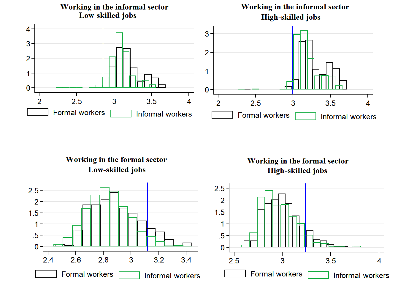
Table 4 reports the corrected predicted average wages for workers working in the formal and the informal sector. Working in the formal sector, formal workers would receive in average higher wages than similar informal sector workers. This gap is statistically significant except for the less than primary education. On the other hand, informal workers working in the informal sector would receive in average higher wages than formal workers with the same observed and unobserved characteristics working in the informal sector. This gap is statistically significant at all levels of education. Also notice that the difference is larger than when working in the formal sector.
Table 4 Predicted wage corrected by employment status
| Working in the formal sector | Working in the informal sector | |||||
|---|---|---|---|---|---|---|
| Characteristics | Formal- sector workers | Informal- sector workers | Mean diff. | Formal- sector workers | Informal- sector workers | Mean diff. |
| Less than primary | 3.085 | 3.079 | 0.006 | 2.779 | 2.758 | 0.021 |
| Primary complete | 3.195 | 3.117 | 0.077*** | 2.886 | 2.832 | 0.054*** |
| Secondary complete | 3.230 | 3.147 | 0.083*** | 2.965 | 2.917 | 0.048*** |
| University complete | 3.390 | 3.264 | 0.126*** | 3.105 | 3.040 | 0.064** |
| Age = 25 to 34 years | 3.141 | 3.068 | 0.072*** | 2.944 | 2.882 | 0.063*** |
| 35 to 44 years | 3.196 | 3.099 | 0.097*** | 2.983 | 2.898 | 0.085*** |
| 45 to 54 years | 3.219 | 3.119 | 0.100*** | 2.979 | 2.897 | 0.082*** |
| 55 to 64 years | 3.393 | 3.170 | 0.223*** | 2.888 | 2.773 | 0.115*** |
Note: * p< 0.1, ** p<0.05, *** p<0.01. Source: Author’s calculation based on 2011 EMOVI.
It can also be observed that age has a nonlinear effect on wages for informal workers, increasing relatively slowly at first, and then decreasing after about age 35. This effect is opposite for workers in the formal sector where a gradually increasing effect is observed.
After controlling for self-selection, on average, if formal-sector workers were artificially allocated to the informal sector, they would have higher wages than similar informal-sector workers in the same informal sector. Intuitively, that is consistent with the idea that formal workers enjoy a significant comparative earnings advantage over informal workers in both sectors, given a particular set of other observed characteristics.
However, this difference is smaller in the informal sector, corroborating the existence of positive self-selection of both formal and informal workers.
Finally, using the corrected estimated coefficients of the two wage equations, we
compute the differences in earnings between formal-and informal-sector employment
for each worker in the simple
Table 5 shows, for the entire sample, the marginal effects at mean of the probability of working in the formal sector. Bootstrapped robust standard errors are reported in parentheses. The coefficient of the wage difference is positive and strongly significant. A larger wage difference between the formal and the informal sector increases the probability of working in the formal sector, after controlling for other individual and family background characteristics.
Table 5 Probability of working in the formal sector for the whole sample
| Model 1 | Model 2 | Model 3 | Model 4 | |
|---|---|---|---|---|
| Earning difference | .0691*** | .110*** | .0850*** | .112*** |
| (7.227) | (9.602) | (8.411) | (10.004) | |
| Age (in years) | .0184** | .0193** | .0205** | .0197** |
| (2.627) | (2.703) | (2.862) | (2.598) | |
| Age squared | -.000304*** | -.000338*** | -.000330*** | -.000343*** |
| (-3.637) | (-3.964) | (-3.849) | (-3.811) | |
| Less than primary completed | Reference | Reference | Reference | Reference |
| Primary completed | .0468 | .0223 | .0329 | .0172 |
| (1.730) | (.739) | (1.181) | (.573) | |
| Secondary completed | .166*** | .116*** | .130*** | .110*** |
| (6.752) | (3.880) | (4.698) | (3.768) | |
| University completed | .513*** | .386*** | .443*** | .380*** |
| (12.976) | (8.274) | (9.752) | (8.192) | |
| 1 if married (d) | .0659* | .0883*** | .0735** | .0866*** |
| (2.520) | (3.330) | (2.793) | (3.316) | |
| 1 if has children (d) | -.0251 | -.0316 | -.0237 | -.0300 |
| (-.813) | (-.991) | (-.761) | (-.994) | |
| Number of chil dren | .00808 | .0125 | .0117 | .0137 |
| (.922) | (1.370) | (1.305) | (1.503) | |
| 1 if father in formal work (d) | .175*** | .178*** | ||
| (8.649) | (8.492) | |||
| Father’s years of schooling | .0165*** | .0120*** | ||
| (6.362) | (3.626) | |||
| 1 if father encouraged his children to study (d) | .0510** | .0491* | ||
| (2.691) | (2.464) | |||
| 1 if father is indigenous (d) | -.0567* | -.00753 | ||
| (-2.017) | (-.170) | |||
| 1 if mother in formal work (d) | .0911* | .0767* | ||
| (2.575) | (1.991) | |||
| Mother’s years of schooling | .0152*** | .00681 | ||
| (5.801) | (1.944) | |||
| 1 if mother encouraged her children to study (d) | .0186 | -.00387 | ||
| (.579) | (-.112) | |||
| 1 if mother is indigenous (d) | -.0749** | -.0625 | ||
| (-2.650) | (-1.356) | |||
| Community size dummies | Yes | Yes | Yes | Yes |
| Region dummies | Yes | Yes | Yes | Yes |
| Observations | 2 837 | 2 837 | 2 837 | 2 837 |
| Log likelihood | -1524.3 | -1458.5 | -1499.4 | -1452.4 |
| McFadden’s R squared | .121 | .159 | .135 | .162 |
| Count R squared (%) | 73.70 | 74.62 | 74.55 | 74.97 |
Log hourly wage difference = ln Yformal−lnYinformal. Controls: Community size dummies: Less than 2 500; 2 500 to 14 999; 15 000 to 99 000; 100 000 or more. Region dummies: North, Center North, Center, Capital, Gulf, South and Pacific. Marginal effects at mean; Bootstrapped robust standard errors in parentheses; (d) discrete change of dummy variable from 0 to 1. *p < 0.10, **p < 0.05, ***p < 0.01. Source: Author’s calculation based on 2011 EMOVI.
In other words, a one percent increases in the ratio of wages (i.e. the wages
that a worker would get in the formal sector, relative to the wage that the same
worker would get in the informal sector) measured by
The coefficient of the schooling variable is positive and significant. This is due to rewarding job opportunities being more readily available to the highly educated workers in the formal sector. The coefficient of marital status confirms that being married increases the probability of working in the formal sector. This result may be a consequence of the workers’ need to provide social security to their families. The number of children at home has no effect.17
Regarding retrospective data conditions when the interviewee was 14 years old, as we expected, having a father who worked in the formal sector has a positive effect on the probability of choosing formal sector. This coefficient is statistically significant in all models. For the entire sample, having a father who worked in the formal sector increases the probability of working in the formal sector by almost 20 percentage points. In addition, we found that a higher level of education for a parent increased the probability of being employed in the formal sector.
6. Conclusions
This paper uses EMOVI 2011 retrospective database for Mexico. Un-like previous surveys in Mexico, this database provides information about family background characteristics in addition to individual and family characteristics. This database allows us to study the effects of a parents formal or informal sector of employment on the son’s formal or informal sector of employment and, in some sense, to contribute to the understanding of intergenerational social mobility in Mexico.
To do this, we use a micro econometric framework based on Lee (1982) to control for the presence of self-selection in the sector of employment decisions. Our results highlight the following aspects. Results suggest positive selection for workers into formal and into informal sectors; significant coefficients show that not correcting for self-selection bias might skew results. This evidence is consistent with the hypothesis that those who have selected a sector of employment possess a comparative advantage for it. A larger wage difference between both sectors increases the probability that workers will choose to work in the formal sector, which provides support for the idea that occupational-sector choice is rational.
With respect to social mobility variables, we find that parents’ schooling is an important vehicle of upward social mobility. This paper corroborates previous literature in Mexico that found that sons tend to follow the same employment sector as their parents, probably through the intergenerational transmission of formal- or informal-sector employment skills.
These findings support the view that investing in better schools and better educational quality, as well as in programs to increase workers human capital such as labor training, will have a positive effect on the acquisition of formal-sector employment skills, and with it, better chances to access formal-sector labor conditions; improving the labor conditions of Mexican workers and the quality of life of their families.
Future research could use life-long longitudinal surveys to fully control for differences in economic conditions facing parents and sons at the time they choose to work. Such differences should have an effect on the decision to work in the formal or in the informal sector.