


 nueva página del texto (beta)
 Inglés (pdf)
 Artículo en XML
 Referencias del artículo
 Enviar artículo por email
 Citado por SciELO
  Similares en
SciELO
Similares en
SciELO 
 Permalink
1. Introduction
Most families in the world consider employment as their main source of income. It is widely recognized that having good opportunities in the labor market is usually associated with keeping poverty away and having better development prospects. At the same time, there is less agreement on which type of employment yields greater levels of development and well-being. There is compelling evidence that a full-time job does not guarantee an individual’s good standard of living. According to the 2013 World Bank Report jobs that promote development are those considered as the most valuable by society. Good jobs can be transformational and offer the best opportunities to attain well-being. This suggests that describing labor-market conditions merely in terms of “employment” and “unemployment” is narrowly focused and in fact limited for most countries in the world. To establish a standard of what a “good job” may be, the International Labor Organization (ILO) proposed the term of “decent work”, which involves four dimensions: a productive and fairly paid work opportunity, security in the workplace, extended social protection, and prospects for social dialogue. Nevertheless, the ILO considers “rights at work” as the basic dimension of work quality thus ignoring important aspects related to the quantity of work. Lugo (2007) identifies two main flaws in the set of indicators traditionally used to study labor market situations. First, the fact that these indicators may not be as relevant for developing countries as they are for developed economies. There is a vast difference in the type of jobs among countries, particularly when differences between formal and informal jobs are taken into account. In developing countries informal jobs are highly segmented by location, economic sector and employment status, thus resulting considerable variations in employment statistics (Chen, Vanek and Carr, 2004; Hussmanns, 2004). Second, these indicators convey a missing link between working conditions and house-hold outcomes that ultimately constitutes an individual’s well-being. In assessing well-being many aspects of our life may be involved, in particular the capacity to achieve a range of functionings in society (Sen, 1993), that is, being able to function in activities that expand the opportunities of what you can do and who you can be. What we should stress here is not only the need to go beyond basic indicators, but also the conflict between distinct inequalities judged in different dimensions (Sen, 1997).
This paper presents an index that considers a series of dimensions and related indicators that characterize the quality and quantity of work, combined with household features that may predispose an individual’s labor situation. The paper focuses on microeconomic aspects of the labor market situation, not denying the significance of macroeconomic dimensions but rather complementing it in order to get a comprehensive image of labor market situations. Our definition of the indicators is broader than traditional approaches used in the labor market literature, such as Lugo (2007), Rodriguez, Cardozo and Parra (2014), Osberg and Sharpe (2005), and Cassar (2010). In order to consider such an array of attributes, we carried out a multidimensional analysis considering persistence and duration of household characteristics that may predispose long-term unemployment. In doing so, we adapted the identification and aggregation steps that Alkire et al. (2014) and Foster (2009) suggest in the chronic poverty analysis to organize long-term employment scarcity data and generate aggregate measures based on well-established principles.
New labor indicators have been proposed aimed at better describing those labor force features that fall outside traditional views of employment and can be used to compare labor markets across countries and regions. Rodriguez, Cardozo and Parra (2014) proposed a territorial labor market development index using equality, productivity and welfare dimensions. Their index explores aspects of development at a local or state level to analyze differences across countries or regions. Osberg and Sharpe (2005, 2002) suggest four dimensions related to economic well-being, where economic security is related to quality and quantity of jobs. The analysis is performed at the country level using an average system of the four dimensions where each component is scaled linearly to the [0,1] interval in order to make level comparisons across or within countries. Also, Schwerdt and Turunen (2007) have developed a quality-adjusted index of labor input within the euro area, also at country level, and have evaluated the significance of changes in human capital for recent developments in productivity growth.
Our analysis diverges from previous indexes in two relevant aspects. First, we construct an index that specifically measures employment deprivation characteristics at an individual level, using house-hold survey information that shows important determinants which are sometimes overlooked in traditional labor market analyses. Second, we focus on long-term aspects of employment deprivation by considering persistence and duration analyses. Here, the analysis differs from the unemployment rate that is basically a one-time “snapshot”. Our index contains the memory of the history of individual experiences similar to the inter-temporal analysis proposed by Shorrocks (2009a, 2009b), yet it is closer to the Foster (2009), and Foster and Santos (2012) approach since we focus on the many dimensions that predispose unemployment status, rather than merely the employment status. Hence, the index we propose combines well-established methodologies traditionally used in chronic poverty analysis, thus allowing both precise comparisons across states and regions, and the identification of important determinants of long-term unemployment.
The structure of the paper is as follows. In section 1 we define the long-term deprivation index in which we identify the long-term deprived and the aggregation of individuals in an overall index. Section 2 discusses the labor market situation in Mexico during the 2007-2014 period of analysis. In section 3 we explains the attributes considered in the analysis, the results and their relation with important labor market employment indicators. Finally, section 5 presents the conclusion.
2. Long-term employment deprivation index
We assume a population of size n, and an individual i having an m -row vector of attributes in time t, x i . The vector constitutes a set of attributes that determine the employment possibilities of an individual i in his/her society. The vector x i is the row of an n × m matrix, x t that describes the society’s individuals characteristics in time t. The jth column of x t , gives the distribution of characteristic j in a society in time t. The entry ij of the matrix x t gives the quantity of characteristics j possessed by an individual i in time t. This array of attributes constitutes the prospects of employment of individuals according to household characteristics in society in time t and can be written as,
In order to measure the long-term unemployment deprivation we follow the poverty measurement methodology proposed by Sen (1976) that involves two stages: identification and aggregation. In the identification stage we seek to determine who is deprived according to those individual’s characteristics that may lead him/her to face lower prospects of employment in society, first in time t and then in a long period of time, which defines the chronic aspect of long-term employment deprivation. The aggregation maps the data of all individuals in society to establish long-term employment deprivation.
To establish long-term employment deprivation we used Alkire et al. (2014) methodology to identify chronically poor people. This identification procedure -also known as the “counting” approach- follows two important characteristics in our analysis. First, it considers several dimensions in the analysis that may reflect different aspects of employment deprivation suffered by individuals. Second, the identification stage proposed here considers the set of attributes in several periods of time as opposed to considering a single period of time- in order to characterize long-term unemployment deprivation status.
According to the identification process, the attributes matrix in (1) follows a series of transformations through which the set of long-term employment deprived individuals can be identified. The first transformation corresponds to the identification of individuals deprived in each dimension of the analysis. To that end, every entry in the column vector x j is compared against a characteristic j threshold in time t that belongs to a vector of thresholds for different dimensions z j t ∈ z t , where individuals having attainments below this limit are considered deprived in that dimension. In this sense, it involves setting up a threshold level where an individual is not falling behind in employment prospects according to a characteristic j. Then we say an individual i is deprived in dimension j if x ij t < z t j but not if x ij t ≥ z t j . The associated matrix of employment deprivations in time t, d t , is given by
Adding the entries in d
t
horizontally yields the number of dimensions in which a person is deprived. The counting approach allows to assign different weights,w
j
∈ w = [w
1
, w
2
,..., w
m
], to the characteristic according to its importance, where
In order to measure long-term employment deprivation we need to take into consideration persistence and duration of household characteristics in several periods of time that may predispose long-term unemployment. In this we follow Foster’s (2009) duration approach that defines a person as chronically poor if he/she remains in poverty for at least a certain number of periods. Similarly, we defined the long-term employment deprived as those individuals who are employment deprived in several periods of time. We refer to τ as the duration cut-off. Then, using the information contained in the employment deprivation spell matrix defined in (3) we now proceed to define the long-term employment deprived counting vector c
LT
, defined as c
LT
= I (k)1
T
, where 1
T
is a T -dimensional vector of ones. The long-term employment deprived counting vector is an n-dimensional vector whose typical element is defined as
Hence, the matrices associated with the long-term employment deprivation can be written as:
2.1. The aggregation procedure
The first stage of the analysis combines different elements of deprivation at the individual level to identify those that are long-term-employment deprived. In this stage, we use a dimensional cut-off k which identifies people that face deprivation in many dimensions, while τ refers to the period of time by which a person is considered long-term employment deprived. The second stage refers to the aggregation of individuals’ information into an index that characterizes the level of long-term employment deprivation in society. There are, however, many ways to complete this aggregation procedure according to certain desirable properties. The simplest measure available is the long-term employment deprivation headcount H LT , which is the fraction of the population that is employment deprived during a period of time τ . The index can be expressed as:
that is, the number of long-term employment deprived q LT , over the total population (n). However, the measure is insensitive to the number of deprivations (Alkire and Foster, 2011) and the number of periods the long-term unemployment deprived experience (Alkire et al., 2014). That is, given the dimensional cut-offs k and τ, if an individual is identified as long-term employment deprived and becomes deprived in the additional dimension of period of time, the long-term employment deprivation headcount does not change.
In order to overcome the limitations of the long-term employment deprivation headcount H LT , we follow Alkire and Foster (2011) and Foster (2009) to obtain a normalized population average of long-term employment deprived. In other words, we add up the means of all dimensions m and periods of time t, to obtain an aggregate index. The proposed dimension and time-adjusted multidimensional deprivation index ED LT , is defined as:
where d
ij
(k) is the deprivation of individual i in dimension j,W
j is the weight assigned to dimension j, such that
where A LT is the average intensity of poverty among the long-term deprived, and D LT the average duration of deprivation among the long-term employment deprived. The ED LT index in formula (7) is the sum of normalized gaps of employment deprivations that predispose individuals’ employment prospects in the labor market, divided by the possible highest value of this sum nm. The total measure can be decomposed into three components: a) the headcount ratio of the population that is employment deprived during a period of time τ ; b) the intensity of deprivation among the long-term employment deprived, in other words, the share of weighted deprivation that long-term deprived people experience in the period in which they are multidimensional employment deprived; c) the average duration among the long-term employment deprived which measures how people experience deficiencies in the labor market. Persistent conditions of insufficiency might severely predispose opportunities in the labor market. The duration of employment deprivation may increase the likelihood of low payment and informal work and hinder opportunities in the labor market in which experience may be relevant. The decomposition allows us to understand the incidence, intensity and duration of those who are long-term employment deprived to better assess the situation in the labor market.
3. Data analysis and labor market in Mexico
Concerning Mexico we used the quarterly employment survey produced by the Mexican National Institute of Statistics, Geography and Informatics (INEGI by its name in Spanish). This survey, which is representative at the state, rural and urban levels, has updated its questionnaire since 2005 and it is currently known as the National Survey of Occupation and Employment (Encuesta nacional de ocupación y empleo, ENOE). The ENOE is a rotating panel that resamples 20 percent of the sample every quarter. In other words, it monitors the individuals for five consecutive quarters. We will work with two sets of five-quarter balanced panels. The periods analyzed are 2007 and 2014, in order to capture the macroeconomic shock of the financial crisis.
Our analysis is limited to the cohort of heads of household aged 24 to 65. We set up the panels with those individuals who received their first questionnaire in the first quarter of the year, and then were resampled in the following two quarters. We were left with 14 070 observations per quarter for the 2007 panel, and 14 257 observations per quarter for the 2014 panel, with attrition rates of 18.85 percent and 18.33 percent, respectively. After further cleaning the data set due to missing data on labor market informality, we are left with 10 699 and 10 461 observations per quarter in 2007 and 2014, respectively.
The survey captures stylized facts of the Mexican labor market. It allows us to know the reason why individuals lost their job, the search mechanisms that workers use to find a job, whether the individual had social security, work benefits or other types of aid, and more. Additionally, it includes demographic characteristics of the individuals that allow us to identify the necessary capabilities for a good performance in the labor market.
3.1. Depiction of the Mexican labor market
Before the 2008 financial crisis, the Mexican labor market was characterized by low unemployment rates, together with high informality and low wages in an economic context of slow growth. After the crisis, though, the levels of unemployment and informality increased (Rodríguez, López and Prudencio, 2013). The government’s response to tackle this shock has been weak (Freije, López and Rodríguez, 2011) and, as in the rest of Latin America, there is an increasing working impoverished population in Mexico (Beccaria et al., 2011; Rodríguez, López and Prudencio, 2013); meaning that for many people having a job is no longer enough to meet their basic needs. Moreover, the level of long-term unemployed in Mexico, although small, has remained the same since the hike of the crisis. In Figure 1 we compare the United States and Mexican unemployment patterns. We present both the short- and long-term levels of unemployment. In the case of the United States both the short- and long-term unemployment levels increased sharply in 2008, but they have decreased almost to pre-crisis levels. That is not the case for Mexico. Both the short- and long-term unemployment levels have stayed relatively the same since the financial crisis.

Sorce: Own calculations using INEGI and Boreau of Labor Stadistics
Figure 1 Unemployment trends in the United State and Mexico
The status of employment -and whether this employment is for-mal or not- varies considerably by gender, level of education, region or industry. We study this further by observing the employment pat-terns presented by the household heads. For Mexico, the status of the household heads in the labor market and their level of education are important determinants of the household’s well-being. At the same time, this group presents a lower attrition rate than other household sub-groups. We thus focused on this group for both the description of the labor market and the construction of the proposed index.
Constructing five period panels for 2007 and 2014, we present in Table 1 the employment distribution of the household heads by different categories. The results presented correspond to panel averages. We observe that most of the male household heads are fully employed, 45.33 percent of them working in the informal market and 39.04 percent in the formal market, while in 2014 these percentages were 42.08 and 38.92, respectively. When considering the underemployed, in 2007, 7.19 percent of men fall into this category, of which 5.97 percent points correspond to those working in the informal market. For 2014, 8.36 percent of men were underemployed, of which 6.94 percentage points were in the informal market. All of these changes between 2007 and 2014 are small, in the range of 1 to 2 percentage points. In the case of women, the biggest proportion of workers is employed in the informal sector, followed by those employed in the formal sector. Once more, most of the underemployed belong to the informal sector. Finally, in contrast to men, in 2007 34.6 percent of female household heads were out of the labor market, and 33.83 percent in 2014.
Table 1 Employment distribution of the household heads by categories
| Employed | Underemployed | Unemployed | Out of the labor market | |||||||||
|---|---|---|---|---|---|---|---|---|---|---|---|---|
| Formal | Informal | Formal | Informal | |||||||||
| 2007 | 2014 | 2007 | 2014 | 2007 | 2014 | 2007 | 2014 | 2007 | 2014 | 2007 | 2014 | |
| Men | 39.04 | 38.92 | 45.33 | 42.08 | 1.22 | 1.42 | 5.97 | 6.94 | 1.73 | 2.57 | 6.71 | 8.07 |
| Women | 26.36 | 25.27 | 33.57 | 33.69 | 0.58 | 0.74 | 3.51 | 4.52 | 1.38 | 1.95 | 34.6 | 33.83 |
| Educ (x<6) | 17.89 | 15.92 | 54.68 | 52.98 | 0.52 | 0.54 | 6.82 | 8.23 | 1.54 | 2.23 | 18.55 | 20.1 |
| Educ (6<x<9) | 40.69 | 36.52 | 40.19 | 40.77 | 1.47 | 1.33 | 5.91 | 7.03 | 2.05 | 2.65 | 9.69 | 11.69 |
| Educ (9<x<12) | 51.08 | 47.52 | 32.03 | 31.52 | 1.46 | 1.78 | 4.17 | 5.08 | 1.51 | 2.5 | 9.75 | 11.6 |
| Educ (12<x) | 57.98 | 57.76 | 29.02 | 25.04 | 1.47 | 1.92 | 2.83 | 3.42 | 1.53 | 2.37 | 7.15 | 9.49 |
| Rural | 17.79 | 15.8 | 58.46 | 58.34 | 0.64 | 0.63 | 7.68 | 9.34 | 1.51 | 2.11 | 13.93 | 13.78 |
| Urban | 39.73 | 39.36 | 39.74 | 36.79 | 1.16 | 1.38 | 5 | 5.83 | 1.68 | 2.48 | 12.7 | 14.16 |
| Primary sector | 8.18 | 6.88 | 81.74 | 80.97 | 0.51 | 0.39 | 9.57 | 11.76 | ||||
| Electricity | 91.39 | 92.19 | 6.85 | 5.92 | 0.93 | 1.78 | 0.83 | 0.12 | ||||
| Manufacturing | 57.53 | 61.48 | 35.43 | 31.11 | 1.92 | 2 | 5.12 | 5.4 | ||||
| Construction | 21.8 | 20.1 | 66.46 | 63.96 | 0.94 | 1.27 | 10.81 | 14.66 | ||||
| Commerce | 32.83 | 37.82 | 59.55 | 53.28 | 1.02 | 1.44 | 6.59 | 7.47 | ||||
| Restaurants | 28.83 | 32.46 | 63.5 | 58.44 | 1.01 | 1.41 | 6.66 | 7.69 | ||||
| Transport | 40.34 | 41.04 | 51.71 | 51.44 | 1.32 | 1.67 | 6.62 | 5.85 | ||||
| Fin. services | 47.86 | 52.67 | 45.56 | 39.43 | 1.57 | 1.62 | 5.01 | 6.29 | ||||
| Other services | 51.55 | 46.73 | 41.7 | 43.97 | 1.18 | 1.61 | 5.57 | 7.69 | ||||
Source: calculations by the authors based on the ENOE.
These results vary significantly when dividing the groups by education level. Individuals with six years or less of education are for the most part fully employed in the informal sector: 54.68 percent in 2007 and 52.98 percent in 2014. Only a small proportion is fully employed in the formal sector, 17.89 and 15.92 percent for the periods analyzed. When considering the household heads with more than 12 years of education, most of them work in the formal sector and are fully employed. Interestingly, the unemployment levels do not vary significantly with the educational level. Nevertheless, the same does not apply with people out of the labor force, which decreases according to the educational achievement of the household head.
When dividing the groups by rural and urban regions we observe that the results from the rural sector are very close to individuals with six years or less of education. Similarly, the patterns of the urban population are parallel to those with higher education.
Finally, when dividing workers by industry we observe a clear lag in the workers employed in the primary sector given that almost all of them work in the informal sector. Workers in the construction industry also present relatively high rates of informality and, along with the primary sectors, these industries present the highest rates of underemployment. Both in regard to informality and underemployment, these groups are followed by workers in commerce, restaurants, and transport. In general, changes between 2007 and 2014 are small when dividing the work force by gender or region (rural/urban), although they are relatively higher when creating subgroups by the level of education or by industry.
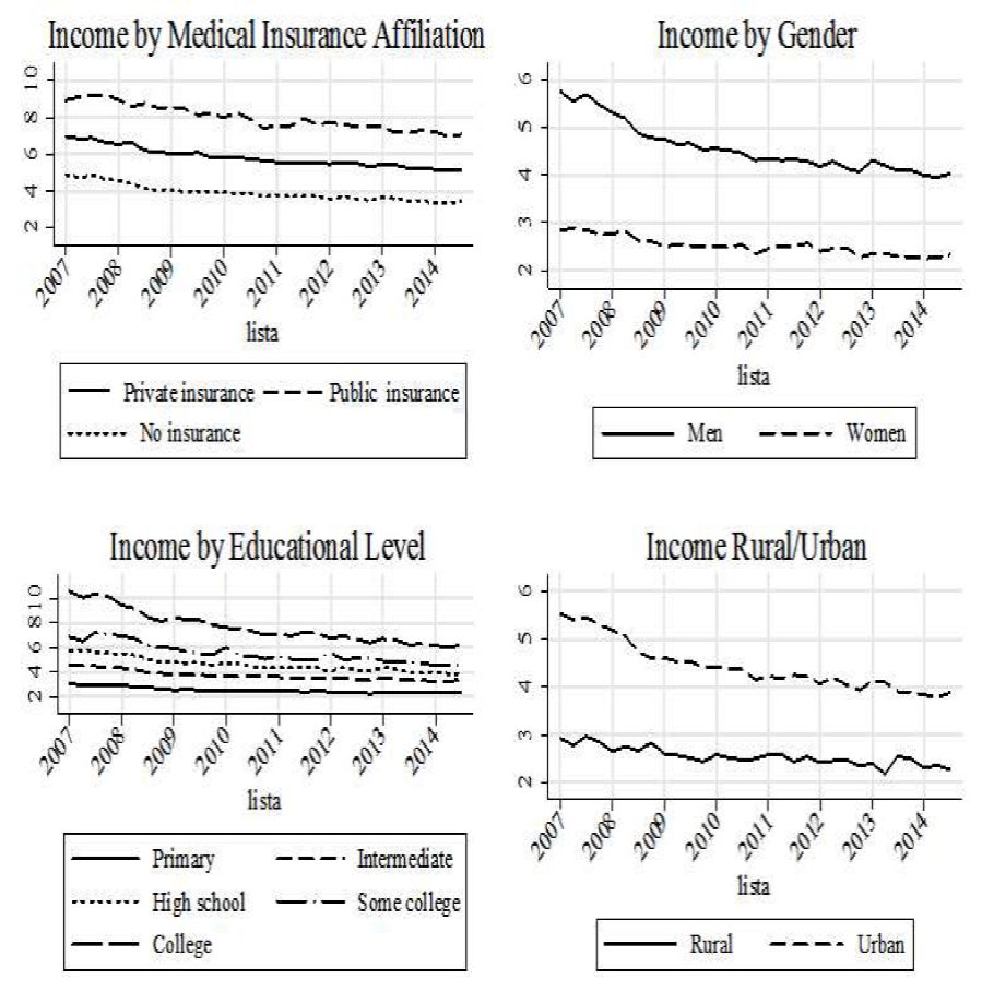
The income trends of these groups, together with the differentiation by medical insurance, reveal a continuing decrease of income in real terms in all sub-groups. Results shown are from panel averages that were constructed for each quarter. For example, data for 2014 first quarter would correspond to a five-quarter panel of individuals whose first observation was in the first quarter of 2014, the panel of the second quarter of 2014 includes those individuals whose first observation was in the second quarter of 2014, and so on. On the horizontal axis we label only the years for clarity. On the vertical axis we report the real income of the household head at 2010 prices. Results are reported in thousands of Mexican pesos.
Finally, Table 2 shows workers’ mobility in the labor market, and how their mobility has changed between 2007 and 2014. In general, mobility decreased during this period, that is, in 2014 a higher proportion of individuals remained in the same status in the labor market. Although fortunate for the employed, the unemployed are striving to find a job. In 2007, before the financial crisis, 9.96 percent of the unemployed remained in that position after five quarters, whereas 74.10 percent of them found a job, 26.69 percent in the formal market and 47.41 percent in the informal market. In contrast, at the beginning of the 2008 crisis the proportion of individuals who were still unemployed amounted to 9.56 percent, but the percentage of those who had found a job decreased to 68.92, the formal market having registered the greatest decrease. Currently, in the 2014 post-crisis period, an even smaller proportion of the unemployed found a job, namely 66.03 percent, mainly due to a hiring decline in the informal market -44.66 percent versus 49.80 percent in 2008-, and secondly due to an increase in people who remained unemployed -12.05 percent vs. 9.56 percent. Moreover, most workers who were already out of the labor force remained in that category and nearly all of those who did manage to enter the labor market found a job in the informal sector.
Table 2 Transition matrix
| 1st quarter of 2007 to 1st quarter of 2008 (pre-crisis period) | |||||
| 107/108 | Formal (%) | Informal (%) | Unemployed (%) | Out of the labor force (%) | Total (%) |
| Formal | 84.52 | 11.14 | 1.55 | 2.79 | 100 |
| Informal | 7.91 | 82.29 | 1.92 | 7.88 | 100 |
| Unemployed | 26.69 | 47.41 | 9.96 | 15.94 | 100 |
| Out of the labor force | 4.14 | 26.19 | 1.38 | 68.29 | 100 |
| Total | 36.80 | 47.73 | 1.86 | 13.61 | 100 |
| 1st quarter of 2008 to 1st quarter of 2009 (hike of crisis period) | |||||
| 108/109 Formal | 82.90 | 12.26 | 1.81 | 3.03 | 100 |
| Informal | 7.53 | 82.18 | 2.44 | 7.85 | 100 |
| Unemployed | 19.12 | 49.80 | 9.56 | 21.51 | 100 |
| Out of the labor force | 2.90 | 23.64 | 1.88 | 71.59 | 100 |
| Total | 35.16 | 48.64 | 2.26 | 14.34 | 100 |
| 1st quarter of 2014 to 1st quarter of 2015 (post-crisis) | |||||
| 114-115Formal | 84.24 | 11.22 | 1.60 | 2.94 | 100 |
| Informal | 8.68 | 80.92 | 2.00 | 8.40 | 100 |
| Unemployed | 21.37 | 44.66 | 12.05 | 21.92 | 100 |
| Out of the labor force | 3.4 | 26.61 | 1.94 | 68.05 | 100 |
| Total | 36.50 | 46.69 | 2.10 | 14.71 | 100 |
Source: own calculations using the ENOE.
In general, unemployment among household heads is low, but as Beccaria et al. (2011) have pointed out, employment may not be sufficient for a household to escape from poverty. The real income of the household heads is decreasing in all the subgroups considered, as well as their mobility in the labor market. In this context, it is important to study the dimensions that may contribute to the resilience of individuals to excel in the labor market and to increase their mobility and well-being. In the following section we describe the dimensions considered in the proposed long-term employment deprivations index.
4. Long-term employment deprivation in Mexico
4.1. Set of labor dimensions
The long-term employment deprivation comprises a set of attributes that characterize different aspects related to individual qualities that offer good opportunities of well-paid jobs in the labor market. We now discuss the choice of attributes, given both their impact for the analysis and the fact that they are subject to specific value judgments. Therefore, it should be discussed as explicitly and as firmly as possible in employment public policy literature. The traditional approach to labor market indicators tends to have a macroeconomic drift and sometimes the indicators are not as relevant in the developing world as they are in developed economies, and hence they do not provide an accurate picture of labor markets in these economies (Lugo, 2007). On the other hand, the World Bank (2013) report on jobs stresses the idea of a “decent job” in which rights and laws serve as a basis to avoid non-decent jobs. This refinement in definition implies that full employment is not the final goal, since a good job is rather that which has the highest value for society.
Recent studies on decent jobs focus on the legal aspects of the activity, which often misrepresent labor market vulnerabilities, even if in most cases they ensure protection (Lugo, 2007). The set of attributes we are interested in are related to the prospect of finding a good job that guarantees an individual’s well-being. A combination of the Lugo (2007) and Rodriguez, Cardozo and Parra (2014), against the backdrop of Alkire et al. (2014) multidimensional poverty selection process was used for outlining the attributes and domain in the analysis. Therefore, our definition is broader that the idea of a “decent” job, as it considers indicators that reflect labor market vulnerabilities and the values and norms of the specific society.
The views of experts inspired our first set of domains and indicators, to which we added household and individual features considered in the literature on decent jobs and labor market indices and the assessment of existing data and data availability. Hence, our list of indicators includes four dimensions and eight indicators, as shown in Table 3.
Table 3 Dimensions
| Category | Dimension | Variable/proxy | Deprivation in dimension (%) | |
|---|---|---|---|---|
| 2007* | 2014* | |||
| Skills/productivity | Deprivation in educational achievement Illiteracy | Dummy if individual is deprived in educational achievement** | 8.75 | 6.14 |
| Illiteracy dummy if an individual in the HH who belongs to EAP is illiterate | 17.64 | 13.92 | ||
| Vulnerability | Working poor | ITLP from CONEVAL | 21.58 | 33.47 |
| Health disability | Dummy if individual is unemployed due to health issues | 0.75 | 0.67 | |
| Security/legal protection | Informality | Dummy if individual is in the informal labor market | 53.33 | 52.18 |
| No contract | Dummy if individual in EAP has no contract | 28.83 | 38.74 | |
| Social cohesion/ access to market | Lack of access to employment benefits*** | Dummy if individual has some kind of benefits | 17.31 | 19.46 |
| Lack of experience | Dummy if accumulated years of experience in the HH are in the first decile of the experience distribution of the population | 10.73 | 10.99 | |
Notes: *Panel averages; ** We define deprivation in education according to CONEVAL (2014) definition; *** It also includes: unemployment aid/liquidation (settlement) of past employment/other. Source: own calculations based on the ENOE.
The percentages presented are for the sample of household heads for the 24 to 65 year-old cohort. Educational achievement is defined as the number of members in a household having completed the schooling years as prescribed by law (primary and secondary level). As we can see, the education deprivation among household heads was 8.75 percent in 2007 and 6.14 percent in 2014. Although deprivation in education decreased, the number of households being working poor increased 12 percentage points in this sample. We define an individual as a working poor if the household’s per capita income that comes from labor is not enough to purchase a basic food basket. Finally, we note that the highest percentages are observed in the category of security and legal protection, which displays the lack of law enforcement concerning the legal requirements to which Mexican workers are entitled.
Table 4 presents various labor market indicators and how they relate to the chosen dimensions. We use five labor market indicators, where U stands for unemployment, UP for unemployment and part-time workers, GP for general pressure in the labor market, defined as the unemployed and the employed who are seeking a job, UND stands for underemployment, and, finally, CCO for workers in critical conditions.1
Table 4 Labor market indicators and deprivation
| Labor market indicators | U* | UP* | GP* | UND* | CCO* | |||||
|---|---|---|---|---|---|---|---|---|---|---|
| 2007 | 2014 | 2007 | 2014 | 2007 | 2014 | 2007 | 2014 | 2007 | 2014 | |
| (%) | ||||||||||
| At least, t > 1 | 5.65 | 7.45 | 13.04 | 15.41 | 18.4 | 22.62 | 25.51 | 28.6 | 26.92 | 29.12 |
| At least, t > 2 | 1.07 | 1.85 | 3.71 | 4.99 | 5.27 | 7.83 | 7.37 | 9.16 | 10.63 | 11.56 |
| At least, t > 3 | 0.28 | 0.42 | 1.3 | 1.63 | 1.65 | 2.34 | 1.63 | 2.67 | 4.36 | 4.98 |
| At least, t > 4 | 0.02 | 0.14 | 0.37 | 0.61 | 0.29 | 0.56 | 0.4 | 0.48 | 1.86 | 2.32 |
| At least, t > 5 | 0.0 | 0.02 | 0.06 | 0.16 | 0.03 | 0.14 | 0.05 | 0.08 | 0.59 | 0.67 |
| Dimension | U ∩ dim | U ∩ dim | GP ∩ dim | U N D ∩ dim | C C O ∩ dim | |||||
| Educational achievement | 8.80 | 5.51 | 12.11 | 8.21 | 7.4 | 5.94 | 11.5 | 8.05 | 18.89 | 13.58 |
| Illiteracy | 18.80 | 12.95 | 26.91 | 19.24 | 14.87 | 13.7 | 21.78 | 18.92 | 35.78 | 27.45 |
| Working poor | 70.00 | 80.39 | 57.02 | 66.6 | 39.69 | 51.08 | 33.57 | 42.41 | 54.15 | 60.25 |
| Health disability | 0.53 | 0.39 | 0.2 | 0.34 | 0.69 | 0.6 | 0.4 | 0.42 | 0.04 | 0.16 |
| Informality | 100 | 100 | 95.13 | 95.98 | 75.07 | 76.71 | 80.95 | 80.1 | 81.84 | 77.05 |
| No contract | 100 | 100 | 57.17 | 64.12 | 57.22 | 64.84 | 35.37 | 40.73 | 29.38 | 38.71 |
| Lack of access to benefits** | 100 | 100 | 54.64 | 60.56 | 49.56 | 51.94 | 27.9 | 29.11 | 21.44 | 25.05 |
| Experience | 13.2 | 12.08 | 9.38 | 11.69 | 14.47 | 15.5 | 9.93 | 11.24 | 6.57 | 6.5 |
Notes: U = unemployed, UP = unemployed and partially employed, GP = general pressure in the labor market, UND = underemployment, and CCO = workers in critical conditions. *Incidence in variables, percentage reported represent the portion of individuals who were in the category indicated at least τ =j . **It also includes: benefits/unemployment aid/liquidation (settlement) of past employment. Source: own calculations using the ENOE.
In the first three rows we report the percentage of individuals that fell under the labor market indicator reference at least t times. For example, for unemployment (U) in 2007, 5.65% of the individuals were unemployed in at least one quarter. This percentage drops when considering individuals who were unemployed durng two quarters, and it is minimal when t = 5. We observe that the 2014 percentages are higher in every category and also that, although the rates of unemployment are low, 29% of workers labored at least one period in conditions considered critical. In line with Joutard and Sagaon (2006), we observe that unemployment in Mexico shows very short durations, which is also the case for the rest of the labor indicators. In this sense, the heads of household seem to be mobile, but many of them fell at one point in time into conditions of labor vulnerability.
For the second part of the table, we take as our sample individuals who fell at least once under the labor market indicator referenced, and then we observed how many of them were at the same time deprived in each of the dimensions specified. For example, all those who were unemployed at least once, 8.80 percent were deprived in the dimension of educational achievement in 2007, and 5.51 percent in 2014. We further note that for the dimension of educational achievement the percentages observed in 2014 are lower than in 2007 despite the fact that the labor market conditions seem to have worsened in 2014. In the rest of the variables, the figure is diverse.
Table 3 shows that 21.58 and 33.47 percent were labor poor in 2007 and 2014 respectively. An individual is considered working poor if the per capita labor income of the household is not sufficient to buy a basic food basket. In Table 4 we observe that of all the house-holds where the head was unemployed, 70 percent were labor poor in 2007, and 80.39 percent in 2014. Those percentages increased when considering other categories, with the only exception being the underemployed. These results are consistent with Inchauste (2012) who argues that status in the labor market is the most important determinant of poverty within the household. Finally, the highest incidences of deprivation correspond to the dimensions of informality and the lack of contract. Note that the percentages presented are panel averages.
4.2. Robustness checks
To check the robustness of the multidimensional index we measured the head count (H LT ) for different cut-offs of k. As expected, there is a reduction in H LT for every increment in the cut-off k. This holds for both the long-term and short-term measures. Here we define the short-term deprived by setting the time dimension cut-off as 1 ≤ τ ≤ 2. The results are presented in the Appendix 1.
When taking k = 3, the levels of the short- and long-term deprived are relatively the same, and a gap of around 20 percent appears when taking k = 2. Also note that long-term deprivation is relatively higher in 2014 than in 2007, and it is also the case for short term deprivation with the exception at k = 1.
Now, when varying both cut-offs k and τ we see a high variability of ED LT ; the results are shown in Table 5. First, when considering the union approach under k = 1 and τ = 1, the incidence of the deprived individuals is as high as 92.13 percent and the adjusted headcount 19.86 percent for 2007. In 2014, we have an increase in incidence to 96.37 and 21.94 percent for the adjusted headcount. At the other extreme, when taking the intersection approach for the time dimension (τ = 5) along with k = 3, we observe that the headcounts are 11.56 and 12.57 percent for 2007 and 2014, and when taking into account the censored headcount we have 5.66 and 6.19 percent.
Table 5 Multidimensional employment deprivation for (k = i, τ = j) and labor market indicators
| Cut-off (τ = j) | Index | Cut-off, k = 1 | Cut-off, k = 2 | Cut-off, k = 3 | Cut-off, k = 4 | ||||
|---|---|---|---|---|---|---|---|---|---|
| 2007 | 2014 | 2007 | 2014 | 2007 | 2014 | 2007 | 2014 | ||
| (%) | |||||||||
| τ = 1 | H LT | 92.13 | 96.37 | 64.53 | 73.29 | 41.84 | 46.55 | 23.87 | 28.95 |
| ALT | 26.56 | 27.20 | 41.89 | 41.77 | 57.47 | 58.39 | 81.10 | 83.17 | |
| DLT | 81.17 | 83.70 | 66.45 | 66.45 | 59.49 | 58.98 | 50.07 | 47.71 | |
| EDLT | 19.86 | 21.94 | 20.34 | 20.34 | 14.31 | 16.03 | 9.69 | 11.49 | |
| τ = 2 | H LT | 80.60 | 92.05 | 49.83 | 59.06 | 30.53 | 33.71 | 14.72 | 17.09 |
| ALT | 26.96 | 27.34 | 40.16 | 40.45 | 52.74 | 53.24 | 68.49 | 69.47 | |
| DLT | 89.92 | 86.69 | 80.36 | 77.64 | 74.12 | 73.82 | 68.76 | 66.94 | |
| EDLT | 19.54 | 21.82 | 16.08 | 18.55 | 11.93 | 13.25 | 6.93 | 7.94 | |
| τ = 3 | H LT | 73.04 | 80.62 | 40.77 | 46.52 | 23.16 | 25.38 | 10.12 | 11.44 |
| ALT | 27.43 | 28.10 | 39.62 | 39.89 | 50.22 | 50.65 | 62.51 | 63.48 | |
| DLT | 95.08 | 93.31 | 89.32 | 87.79 | 84.99 | 84.91 | 81.82 | 80.25 | |
| EDLT | 19.05 | 21.14 | 14.43 | 16.29 | 9.88 | 10.92 | 5.17 | 5.82 | |
| τ = 4 | H LT | 67.38 | 71.59 | 33.56 | 37.17 | 17.38 | 19.06 | 7.01 | 7.43 |
| ALT | 27.92 | 28.94 | 39.66 | 40.01 | 49.00 | 49.35 | 59.25 | 59.85 | |
| DLT | 98.03 | 97.51 | 95.62 | 94.78 | 93.30 | 93.18 | 91.47 | 91.15 | |
| EDLT | 18.44 | 20.21 | 12.72 | 14.09 | 7.94 | 8.76 | 3.80 | 4.05 | |
| τ = 5 | H LT | 60.77 | 62.70 | 26.22 | 27.47 | 11.56 | 12.57 | 4.02 | 4.14 |
| ALT | 28.54 | 29.96 | 40.32 | 40.99 | 49.01 | 49.30 | 56.86 | 57.87 | |
| DLT | 100 | 100 | 100 | 100 | 100 | 100 | 100 | 100 | |
| EDLT | 17.34 | 18.79 | 10.57 | 11.26 | 5.66 | 6.19 | 2.29 | 2.40 | |
| 2007* | 2014* | ||||||||
| Unemployment rate | 1.40 | 1.98 | |||||||
| Part time workers and unemployed | 3.69 | 4.56 | |||||||
| Unemployed and employed who searched for a job | 5.13 | 6.70 | |||||||
| Underemployment rate | 6.99 | 8.20 | |||||||
| Workers under critical circumstances | 8.88 | 9.73 | |||||||
Notes: *Panel averages, Source: own calculations based on the ENOE.
When observing both the intensity A LT and the duration D LT indexes, we note that the duration is relatively high throughout the table, whereas A LT varies more. From now on we will use the cut-off of k = 3 and τ = 3.
Now, considering the second part of Table 5, using the chosen cut-offs we observe that the index does not follow the unemployment rate closely. Nevertheless, it does approximate considerably to the rest of the labor market indicators, which are more related to either the level of satisfaction of the individual in the labor market, or the definition of the precariousness of work in general. In other words, ED LT as a measure seems to resemble the capabilities of the individual to work at non-precarious jobs. In Figure 3, we estimate the headcount H LT for each quarter from 2007 to 2014 using the cut-offs of k = 3 and τ = 3, and we compare it to the levels of unemployment and underemployment, and workers in critical conditions. As can be attested, there are also similar patterns in the level of H LT and the level of workers in critical conditions in the period under examination.

Now, to further analyze the behavior of each dimension and its relative importance in ED LT , Table 6 exhibits the censored head-counts of each dimension and their respective relative influence for various cut-offs of τ .
Table 6 Multidimensional long term employment deprivation for τ = j, k = 3
| 2007* | 2014* | Changes (2007, 2014) | |||||||
|---|---|---|---|---|---|---|---|---|---|
| τ = 1 | τ = 3 | τ = 5 | τ = 1 | τ = 3 | τ = 5 | τ = 1 | τ = 3 | τ = 5 | |
| (%) | |||||||||
| H LT | 41.84 | 23.16 | 11.56 | 46.55 | 25.38 | 12.57 | 4.71 | 2.22 | 1.01 |
| ALT | 57.47 | 50.22 | 49.01 | 58.39 | 50.65 | 49.30 | 0.92 | 0.43 | 0.29 |
| DLT | 59.49 | 84.99 | 100 | 58.98 | 84.91 | 100 | -0.51 | -0.08 | 0.00 |
| EDLT | 14.31 | 9.88 | 5.66 | 16.03 | 10.92 | 6.19 | 1.72 | 1.04 | 0.53 |
| Censored headcount | |||||||||
| Educ. achievement | 8.01 | 6.90 | 5.54 | 5.78 | 5.10 | 4.15 | -2.23 | -1.79 | -1.39 |
| Illiteracy | 15.24 | 11.91 | 8.23 | 12.78 | 10.57 | 7.53 | -2.45 | -1.34 | -0.69 |
| Working poor | 14.00 | 9.83 | 5.85 | 20.63 | 13.35 | 7.76 | 6.63 | 3.52 | 1.91 |
| Health disability | 0.42 | 0.23 | 0.14 | 0.39 | 0.18 | 0.10 | -0.02 | -0.06 | -0.04 |
| Informality | 21.39 | 14.41 | 7.20 | 26.72 | 17.38 | 8.75 | 5.34 | 2.98 | 1.55 |
| No contract | 34.06 | 21.38 | 11.24 | 36.65 | 23.49 | 12.33 | 2.59 | 2.12 | 1.09 |
| Lack of benefits | 16.71 | 12.21 | 6.21 | 19.06 | 14.22 | 7.47 | 2.35 | 2.01 | 1.26 |
| Experience | 4.66 | 2.24 | 0.92 | 6.24 | 3.07 | 1.48 | 1.58 | 0.83 | 0.57 |
| Relative weight | |||||||||
| Educ. achievement | 7.00 | 8.72 | 12.23 | 4.51 | 5.84 | 8.38 | -2.49 | -2.88 | -3.85 |
| Illiteracy | 13.31 | 15.05 | 18.14 | 9.96 | 12.10 | 15.19 | -3.34 | -2.95 | -2.95 |
| Working poor | 12.23 | 12.42 | 12.91 | 16.08 | 15.28 | 15.66 | 3.86 | 2.85 | 2.74 |
| Health disability | 0.37 | 0.30 | 0.32 | 0.31 | 0.20 | 0.20 | -0.06 | -0.09 | -0.12 |
| Informality | 18.68 | 18.22 | 15.87 | 20.84 | 19.90 | 17.64 | 2.15 | 1.68 | 1.77 |
| No contract | 29.75 | 27.02 | 24.80 | 28.57 | 26.89 | 24.87 | -1.17 | -0.13 | 0.08 |
| Lack of benefits | 14.60 | 15.44 | 13.71 | 14.86 | 16.28 | 15.07 | 0.26 | 0.84 | 1.36 |
| Experience | 4.07 | 2.83 | 2.02 | 4.87 | 3.51 | 2.99 | 0.79 | 0.68 | 0.97 |
Note: *The percentages are panel averages. Source: calculations by the authors based on the ENOE.
In addition, we also present the change observed from 2007 to 2014. In general, the dimensions of working poor, informality, lack of contract, lack of benefits, and experience have worsened, whereas the dimensions of educational achievement, illiteracy, and health disability have improved. Nevertheless, as observed in the changes presented, the differences between the two panels are small, with the exception of the working poor and the informality levels when considering τ = 1. When observing the relative importance of each dimension, the most important variables in both periods were lack of contract and informality, followed by illiteracy and working poor. Interestingly, the relative importance of the variables related to productivity, which are education achievement and illiteracy, decreased the most, and the variable that fared the worst was working poor.
Finally, making use of the sub-group and decomposition properties of the Alkire et al. (2014) measure, we estimated the results for each state. Using the cut-offs of k = 3 and τ = 3, we generated deprivation maps by state for the variables H LT A LT and E D LT in Figure 4.

For the measure of ED LT , the 2007 map generates a clear division between the northern, central and southern regions. The lighter colors represent higher levels of deprivation. Therefore, we observe that workers in the north are less deprived than those in the central and southern regions. The state that performed the worst was Chiapas. In 2014, these divisions were less strong, mainly due to a deterioration in the labor characteristics of the workers in the states of Chihuahua and Coahuila.
The maps for the headcount H LT A LT and D LT can be found in Appendix 2. For the former we observe, on the one hand, that in 2007 the more prosperous northern region, along with Mexico City, presented the lowest levels in the head count (H LT ). On the other hand, the southern border had the worst performance. In 2014 the figure changes slightly, and some states in the north -as we pointed out before- presented a deterioration in their labor market conditions, reflected in higher levels of H LT .
The picture for the intensity in deprivation is varied. In 2007 the state of Tabasco performed the worst in this category, and for 2014, the state of Puebla. Finally, in regard to duration, the south presents the longest spells of deprivation both in 2007 and 2014.
5. Conclusions
In this paper we suggest a new approach for measuring long-term employment deprivation. It considers a series of dimensions and associated indicators that characterize the quality and quantity of work, combined with household features that may predispose an individual’s labor situation. The analysis considers time and its chronicity since it focuses on long-term aspects of employment by analyzing its persistence and duration. Hence, it provides both conceptual and empirical value, as traditional macroeconomic analysis is enriched by attaching importance to the microeconomic aspects of the labor market context.
Based on the 2007 and 2014 Encuesta nacional de ocupación y empleo (ENOE), this study examines the long-term deprivation status of persons in Mexican states. When analyzing the censored head-counts of each dimension and its respective influence we found that the most important variable is lack of contract and informality. On the other hand, the variables associated to productivity have a lower relative importance. We map the long-term deprivation measure and observe that the north is less deprived than the central and southern regions. However, during 2014 this division was less significant mainly due to the deterioration in the labor characteristics of the workers in the states of Chihuahua and Coahuila. We found that the index proposed does not closely follow traditional unemployment rates but is rather associated with the characterization of precariousness of work in general. This discrepancy with the traditional unemployment rate highlights the fact that long-term deprivation status is a multidimensional phenomenon that may plausibly be measured in several distinct ways.


