


 nueva página del texto (beta)
 Inglés (pdf)
 Artículo en XML
 Referencias del artículo
 Enviar artículo por email
 Citado por SciELO
  Similares en
SciELO
Similares en
SciELO 
 Permalink
1. Introduction
The Republic of Korea, generally identified as one of the Asian tigers, has received much attention due to its phenomenal growth in recent decades. For some, this is the result of market-friendly policies (see Westphal, 1978, Krueger, 1979 and World Bank, 1993); for others, it derived from the actions taken by “the developmental state” (see Amsden, 1989, Haggard, 1990 and Woo-Cumings, 1999). Its growth strategy has sometimes been oversimplified and described as an exportled growth model, as if Korea’s success could be solely explained by its export promotion. While the Korean government did indeed actively promote exports during the 1960s and 1970s, its development policy was much more complex and farreaching (Chang, 1994).
The variety of policies implemented and the particularities of the Korean economy generated a particular causal relationship between economic growth and the external sector. This process was the result of a successful strategy that consisted in fostering the creation and development of competitive firms, so they could achieve world-class status. Once they reached such a level, Korean firms did not need as much protection as those of other countries; exports came as a natural result of their level of efficiency. Korea’s success should not be seen as the expected outcome of a liberalization process, but rather as the result of a specific development strategy applied step by step under these specific circumstances. In order to give a better explanation of the causality effects found in the quantitative analysis, we begin with a brief historical review of the development and industrial policies carried out by the Korean government, focusing on those that are related to the external sector, as well as of some key points of its liberalization process.
The Korean economy has shown consistent real GDP per capita growth (5.24% average annual real growth from 1950 to 2015). The economic policies carried out by Korea have transformed the country from a rural economy into an industrialized one, through the most rapid developing process that any country has ever experienced. Given its results, the Korean case must constitute an example of policies to be considered by a developing country (see Figure 1).

Source: Conference Board (2015).
Figure 1 Annual GDP per capita in 1990 US$ (converted at geary khamis PPPS)
Misleadingly, Korea has been described as an example of the exportled growth model. As we can observe in Figure 2, Korea’s international trade, expressed in terms of real exports and imports, has grown enormously over the last decades. As a frame of reference, Korea’s real exports in the second quarter of 2014 were 13 times those of the first quarter in 1980, while imports grew 8 times during the same period. Indeed, although the fast economic growth in Korea was accompanied by rapid growth in exports, we shall not rush into conclusions about the direction of causality.

Source: authors’ calculations using OECD (2016a) data.
Figure 2 Real exports and imports (in millions of US$-standardized to the year 2000)
Following the Japanese example, one of the key characteristics of the Korean strategy was to limit the access of foreign direct investment (FDI) to the Korean economy, although it was forced to partially liberalize after the Asian crisis in the nineties. Consequently, FDI experienced a rapid growth after the 1997 crisis and changes in regulation, but stagnated after 2000, within a narrow range of variability (see Figure 3).

Source: authors’ calculations using OECD (2016a, 2016b) data.
Figure 3 Real foreign direct investment inflows
The purpose of this study is to analyze the causal relationships between the Korean foreign sector and its economic growth and to test the traditional hypothesis of the sources of economic growth. We do that by estimating and analyzing a VAR (vector autoregresion) model with four variables (GDP, exports, imports and FDI), since the 1980s. The study tests the long-run and short-run relationships between GDP, exports, imports and FDI for Korea from 1980Q1 to 2015Q1 using quarterly data. This paper contributes to the debate on the sources of Korea’s economic growth, as well as to the literature on the connection between economic growth, trade liberalization and industrial policies.
Our methodology is close to that used by Nguyen (2011), who implements a set of econometric procedures, including the unit root test of four series, lag structure, the VAR diagnostic, the Johansen co-integration test, the Granger Causality/Block Exogeneity Wald Test (GCBEW test), analysis of impulse response and analysis of variance decomposition, to study the impact of trade liberalization on Malaysian and South Korean economic growth using annual data. This methodology is relevant for our study for two reasons. First, it has the advantage of avoiding misspecification and minimizing the resulting omitted-variables bias. Second, it allows us to test and estimate the causal relationship among variables (GDP, exports, imports and FDI) through a four-variable VAR model.
The remainder of the paper is organized as follows. The second section presents a brief literature review. The third describes the data set. The fourth section explains the methodology as well as the estimation results. The conclusions are given in the fifth section.
2. Literature review
Korean industrialization took off under the rule of Park Chung-hee, who, through an intense industrial policy, created rents in order to promote selected sectors. Together with protectionist policies, the government promoted exports both to finance the necessary imports and as a measure of the improvement in competitiveness of firms, in order to justify the access of these firms to subsidies and a protected national market.
After the death of Park Chung-hee and the short-lived government of Choi Kyu-hah, Chun Doo-hwan took power through a coup d’etat in 1980 and began a slow process of liberalization, which minimized its potential negative impact. Korea still kept some of the institutions that were created following the logic of the developmental state, such as the Korean Trade Promotion Corporation (KOTRA). Current president Park Geun-hye’s strategy of promoting the creative economy shows that the Korean interventionist industrial policy did not disappear with the arrival of democracy nor with the 1997 crisis. In any case, even though the rapid economic growth of the liberalizing period starting in 1980 must be seen as the consequence of the policies adopted during Park Chung-hee’s regime, those periods should not be analyzed together due to the high degree of intervention of his policies.
Trade liberalization may have a negative impact on developing countries because of the increase of imports, which worsen the trade balance (Santos-Paulino and Thirlwall, 2004). The magnitude of the impact on exports or imports depends on the country and on its initial conditions, as shown by Awokuse (2007).
Since the 1970’s, there has been a considerable shift towards export promotion strategies in most of the developing world, supported by the idea that export expansion leads to better resource allocation, “creating economies of scale and production efficiency through technological development, capital formation, and employment generation” (Shirazi and Abdul-Manap, 2005: 472). The success of the outward-oriented policies of the East Asian Tigers provoked a great deal of consensus over the exportled growth hypothesis. It was not just accepted by academicians (see Feder, 1983 and Krueger, 1980), but it evolved into a “new conventional wisdom” (Tyler, 1981, Balassa, 1985). Several countries followed these policy recommendations, which were also promoted by institutions the World Bank (1987).
However, the exportled growth hypothesis has been questioned in recent times. Ahmad and Harnhirun (1995) did not find a good basis to confirm the hypothesis of exportled growth for the ASEAN region (Indonesia, Malaysia, the Philippines, Singapore and Thailand). Instead, they claimed that the interaction of exports with interior mechanisms could be a more suitable explanation for the economic growth of these countries.
Although imports could, at least theoretically, increase growth because of the access to a greater market of intermediate inputs and the improvement of competitiveness, they can also destroy the domestic productive chains, reallocating the domestic resources from productive employment to unemployment.
The cautious observations of liberalization processes and the dynamics between growth and the external sector in different countries, especially the Asian ones, are of great importance for Latin American countries. They are of particular interest for countries such as Mexico, Argentina, Brazil, Peru and Uruguay, where the twentieth century saw a significant increase in the elasticity of the ratio of exports and imports with respect to income, (Guerrero de Lizardi, 2006).
FDI is, along with exports and imports, a key variable in explaining the relationship between a country and its external sector. When purchasing goods abroad, companies can, basically, decide between importing those goods or producing them in the foreign country, depending on the comparative advantages of either option. Companies face a similar choice between investing in a foreign country and exporting their goods to such market. Because of these substitutabilities, FDI has also been studied, along with foreign trade, to determine its relationship with economic growth. The choice between exports and FDI depends on the level of convenience, risk, profit and long-run developing strategy of firms, competitors, etc. (Liu, Wang and Wei, 2001). Although FDI may increase capital and, therefore, production, it may also crowd-out domestic firms, so its total effect in developing countries might be negative (see Herzer, 2012).
There are a significant number of studies on the relation between economic growth, export and FDI. Jung and Marshall (1985) perform causality tests between exports and growth for 37 developing countries; the results cast considerable doubt on the validity of the export promotion hypothesis. Henriques and Sadorsky (1996) investigate the exportled growth hypothesis for Canada by constructing a vector autoregression (VAR) in order to test for Granger causality between real Canadian exports, real Canadian GDP, and Canada’s real terms of trade; they find that these variables are co-integrated and evidence of a one-way Granger causal relationship in Canada whereby changes in GDP precede changes in exports (i.e. growth-driven exports hypothesis). Zestos and Tao (2002) study the relations between the growth rates of exports, imports, and the GDP, for the 1948-1996 period for Canada and the United States, finding bidirectional causality for Canada from the foreign sector to GDP and vice versa, and a weaker relationship between the foreign sector and GDP for the United States.
Kónya (2004) investigates the possibility of exportled growth and growth-driven export by testing for Granger causality between the logarithms of real exports and real GDP in twenty-five OECD countries with annual data for the 1960-1997 period, and finds mixed results.1 Shirazi and Abdul-Manap (2005) examine the exportled growth hypothesis for five South Asian countries through cointegration and multivariate Granger causality tests, and they also find mixed results.2 Liu, Shu and Sinclair (2009) look for causal relationships between foreign trade, FDI and growth in a panel of Asian economies and reject any of the considered variables to be exogenous. Our paper is methodologically close to that of Nguyen (2011), who analyzes the impact of trade liberalization on economic growth for Malaysia and South Korea; he uses a four variable vector autoregression (VAR) to study the relationship between trade, FDI and economic growth over the time period from 1970 to 2004 (for Malaysia) and from 1976 to 2007 (for Korea). Unlike Nguyen, we do not consider data from the 1970’s, since the Fourth Republic was a very interventionist period in Korea. The exclusion of those years is more than compensated for by the use of quarterly data, which enriches the sample.
We coincide on denying any causal relationship from FDI on any of the other variables and on the negative impact of imports on GDP. Unlike Nguyen, we find a positive causal relationship from GDP on both exports and imports. Also contrary to Nguyen, we do not find causal relationships from GDP on FDI, neither from exports on FDI or GDP. According to the last one, we would reject the exports-led gwroth hypothesis for Korea, which might have important implications for countries such as Mexico. It might be the case that the data from the highly intervened 1970s explained the absent causalities. FDI seems to consolidate in Korea as a substitute of imports. It could also be the case that the causalities found by Nguyen are driven by a data set (1976-2007) that contains, relatively to its size, a higher proportion of institutional changes, such as changes in trade policy.
3. The data set
We use quarterly data from Q1-1980 to Q1-2015. The four time series are (see Figure 4):
LRGDP (logarithm of real GDP)
LREXP (logarithm of real exports)
LRIMP (logarithm of real imports)
LRFDIL (logarithm of real FDI liabilities).

The data has been sourced from the OECD (2016a, 2016b) statistics. In order to express them in real terms, we have taken the series in current prices and transformed them by using a GDP deflator, so that all variables were expressed in millions of 2000 US dollars before taking logs. Due to the high volatility of FDI, when analyzing quarterly data, we have considered the average FDI of the last four periods before taking logs.
4. Estimations
In this section, we estimate the relationships among the four variables. In order to do so, we follow Nguyen (2011) and perform the following steps:
Unit root test of four time series
Test the lag-length of the VAR model
Estimate four variable VAR model
VAR diagnostics (residual autocorrelation and residual normality tests)
Johansen cointegration test
Granger causality Wald test
Dynamic simulation (impulse response function and variance decomposition).
4.1. Estimation, tests and Granger causality
We begin by implementing a unit root test on our four series (LRGDP , LREXP , LRIMP and LRFDIL) by using the Phillip-Perron test. If all series are found to be I(1), they will be used in a four variable VAR. Table 1 and Table 2 provide the evidence that the four time series are non-stationary of order one.
Table 1 Philips-Perron test (levels)
| Variables | Intercept | Trend and intercept |
|---|---|---|
| LRGDP | -5.4178 | -1.1821 |
| LREXP | -1.1747 | -2.7393 |
| LRIMP | -0.8241 | -2.9459 |
| LRFDIL | -2.7817 | -1.9240 |
Note: the critical values for the PP test with intercept and with trend and intercept at the 1%, 5% and 10% significance levels are respectively: -3.4785, -2.8826, -2.5781; -4.0264, -3.4430, -3.1462.
Table 2 Philips-Perron test (first differences)
| Variables | Trend and intercept |
|---|---|
| LRGDP | -10.0479 |
| LREXP | -10.6823 |
| LRIMP | -9.8883 |
| LRFDIL | -12.9157 |
Note: the critical values for the PP test at the 1%, 5% and 10% significance levels are: -4.0269, -3.4432, -3.1463.
The results from unit root tests in levels reported in Table 1 show that for most tests we cannot reject the null hypothesis (non-stationary) at a 0.01 significant level. LRGDP is clearly growing over time (see Figure 4) so the appropriate test requires to inclusion of a trend and intercept (Elder and Kennedy, 2001). Thus, all the variables have a unit root and we need to test the unit root of their first difference.
Since their absolute values are higher, in absolute values, than the 1 percent critical level, we can reject the null hypothesis of non-stationary. Thus, we can conclude that the four series in levels are non-stationary with the root of order 1 (for robustness: see the results of the standard Augmented Dickey-Fuller (ADF) and Dickey-Fuller tests for Generalized Least Squares (DFGLS) in Appendix). There-fore, we can proceed to construct a four-variable VAR model. Now, following Shin and Pesaran (1998), consider a four-variable (unstructured form) standard VAR model of order p as:
where y t = (LRGDP, LRE X P, LRI M P and LRF DI L) is a 4 × 1 random vector; A i is 4 × 4 fixed coefficient matrix; p is order of lags; x i is a d × 1 vector of exogenous variables; B is a 4 × d coefficient matrix; and e t 4 × 1 vector of error terms. As exogenous variables, we use nine dummy variables which ensure the normality of errors:
The first five refer to political events: the effects of the instability of the creation of the Fifth Republic (1981Q3); the arrival of FDI related to the Asian Games and preparation for the Olympic Games (1986Q1); the end of the Fifth Republic (1988Q1 and 1988Q2) and political instabilities related to the demand for a greater democratization (1989Q1). The last four are related to the 1997 Asian financial crisis (1998Q1 and 1998Q2) and global financial crises (2008Q4 and 2009Q1).
As claimed by Shin and Pesaran (1998) and Nguyen (2011), we are making the following assumptions:
Assumption 1: E [ε t ] = 0, E [ε t ε ʼ t ] = , while E [ε t ε ʼ t0 ] = 0 when t = t ʼ and E [ε t /w t ] = 0.
Assumption 2: All the roots lie outside the unit circle.
Assumption 3: y t−1 , y t−2 ...y t−p , x t ... are not perfectly collinear
In addition to the selection of the lag order we will test for VAR residual serial correlation and normality (Nguyen, 2011).
We constructed the VAR system with four endogenous variables (LRGDP, LRE X P, LRIM P and LRF DI L) and nine dummy variables to obtain normality in the residuals. The result from the test for lag length criteria, based on the four-variable VAR system with the maximum lag number of 10, is reported in Table 3. The lag order chosen by FPE criteria is 5. In addition to this information, we implemented the VAR residual correlation LM test and the residual normality test (Lutkepohl, 2005). An appropriate lag order needs to satisfy those tests.
Table 3 Test for lag length criteria
| Lag | LogL | LR | FPE | AIC | SC | HQ |
|---|---|---|---|---|---|---|
| 0 | 12.51564 | NA | 1.03e-05 | -0.133057 | -0.043931 | -0.096845 |
| 1 | 846.8335 | 1603.455 | 2.88e-11 | -12.91927 | -12.47364* | -12.73821* |
| 2 | 859.7092 | 23.94073 | 3.03e-11 | -12.87046 | -12.06832 | -12.54455 |
| 3 | 877.4405 | 31.86087 | 2.95e-11 | -12.89751 | -11.73887 | -12.42675 |
| 4 | 895.2069 | 30.81370 | 2.88e-11 | -12.92511 | -11.40997 | -12.30950 |
| 5 | 918.1753 | 38.40032* | 2.60e-11* | -13.03399 | -11.13234 | -12.27353 |
| 6 | 934.2457 | 25.86325 | 2.62e-11 | -13.03509* | -10.80694 | -12.12978 |
| 7 | 940.5769 | 9.793610 | 3.08e-11 | -12.88401 | -10.29936 | -11.83386 |
| 8 | 952.2245 | 17.28943 | 3.35e-11 | -12.81601 | -9.874852 | -11.62100 |
| 9 | 969.8641 | 25.08124 | 3.33e-11 | -12.84163 | -9.543966 | -11.50177 |
| 10 | 988.6808 | 25.57894 | 3.27e-11 | -12.88564 | -9.231473 | -11.40093 |
Note: *indicates lag order selected by the criteria.
The maximum lag length of the criteria differs among them. We have run the VAR model for lag orders 1, 6 and 10 and applied the LM and Normality tests, but failed to find a clear answer. The results of the VAR model with lag 1 satisfy the normality test and the autocorrelation at 1%. Although the estimations with lag orders of 5 and 6 show a slight improvement of the autocorrelation statistics, the errors behave non-normally. Moreover, according to Liew (2004), the Hannan-Quinn information criterion (HQ) has the highest probability of a correct estimation for sample sizes greater than 120. Based on that, we proceed by estimating the VAR model with lag order of 1.
As we can see in Table 4, the high value of the adjusted coefficient of determination and the low value of the determinant of the residual covariance matrix are positive results. On the other hand, the sum of squared residuals seems to be high in the case of LRF DI L. The results from the VAR residual normality test are reported in Table 5.
Table 4 VAR model whit 1 lag and 9 dummy variables
| Lag | LRGDP | LREXP | LRIMP | LRFDIL |
|---|---|---|---|---|
| R-squared | 0.999750 | 0.997239 | 0.996677 | 0.988226 |
| Adj. R-squared | 0.999723 | 0.996947 | 0.996326 | 0.986981 |
| Sum sq. resids | 0.012272 | 0.239261 | 0.263819 | 0.691995 |
| S.E. equation | 0.009989 | 0.044105 | 0.046313 | 0.147940 |
| F-statistic | 37774.06 | 3416.773 | 2838.111 | 794.1120 |
| Log likelihood | 444.0540 | 240.5928 | 233.8997 | 74.78795 |
| Akaike AIC | -6.278160 | -3.307924 | -3.210215 | -0.887442 |
| Schwarz SC | -5.979768 | -3.009531 | -2.911822 | -0.589049 |
| Mean dependent | 13.36036 | 12.27962 | 12.23782 | 6.500733 |
| S.D. dependent | 0.600286 | 0.798168 | 0.764083 | 1.296581 |
| Determinant residual covariance (dof adj.) | 5.58E-12 | |||
| Determinant residual covariance | 3.63E-12 | |||
| Log likelihood | 1026.922 | |||
| Akaike information criterion | -14.17404 | |||
| Schwarz criterion | -12.98047 | |||
Table 5 VAR residual normality test
| Component | Skewness | Chi-sq | df | Prob. |
|---|---|---|---|---|
| LRGDP | 0.066306 | 0.100387 | 1 | 0.7514 |
| LREXP | 0.026598 | 0.016154 | 1 | 0.8989 |
| LRIMP | 0.087018 | 0.172896 | 1 | 0.6776 |
| LRFDIL | -0.171155 | 0.668880 | 1 | 0.4134 |
| Joint | 0.958317 | 4 | 0.9160 | |
| Component | Kurtosis | Chi-sq | df | Prob. |
| LRGDP | 3.648368 | 2.399672 | 1 | 0.1214 |
| LREXP | 3.307800 | 0.540814 | 1 | 0.4621 |
| LRIMP | 3.146348 | 0.122259 | 1 | 0.7266 |
| LRFDIL | 3.639561 | 2.334924 | 1 | 0.1265 |
| Joint | 5.397669 | 4 | 0.2489 | |
| Component | Jarque-Bera | df | Prob. | |
| LRGDP | 2.500059 | 2 | 0.2865 | |
| LREXP | 0.556968 | 2 | 0.7569 | |
| LRIMP | 0.295155 | 2 | 0.8628 | |
| LRFDIL | 3.003804 | 2 | 0.2227 | |
| Joint | 6.355985 | 8 | 0.6074 | |
Given the results shown in from Table 5, we cannot reject the hypothesis of normality, since all individual Chi-square values for skewness and kurtosis are lower than the critical value
Table 6 shows that we cannot reject the null hypothesis of no autocorrelation up to lag 12, since the values of the LM-Statistics for the lag order of 1, 2, 3, 4,...12, are all lower than the critical value
Table 6 VAR residual serial colrrelation LM test
| Lags | LM-Stat | Probabilities from Chi-square with 16 degrees of freedom |
|---|---|---|
| 1 | 12.39986 | 0.7160 |
| 2 | 26.56133 | 0.0466 |
| 3 | 26.06180 | 0.0532 |
| 4 | 31.40808 | 0.0119 |
| 5 | 18.84123 | 0.2770 |
| 6 | 11.77191 | 0.7595 |
| 7 | 12.34180 | 0.7201 |
| 8 | 18.60542 | 0.2897 |
| 9 | 8.187881 | 0.9431 |
| 10 | 15.09080 | 0.5180 |
| 11 | 17.98524 | 0.3248 |
| 12 | 8.330402 | 0.9384 |
To test the long-run cointegration relationship between the four time series, we carried out the Johansen (1995) cointegration test. In order to do so, we first choose the appropriate lag criteria for the cointegration test. The results of the VAR order selection are given in Table 7.
Table 7 Test for lag length criteria of the cointegration test
| Lag | LogL | LR | FPE | AIC | SC | HQ |
|---|---|---|---|---|---|---|
| 0 | 1.982275 | NA | 2.07e-05 | 0.563226 | 1.424048 | 0.913040 |
| 1 | 1016.661 | 1818.906 | 7.77e-12* | -14.23202* | -13.02687* | -13.74228* |
| 2 | 1024.950 | 14.36752 | 8.74e-12 | -14.11778 | -12.56830 | -13.48812 |
| 3 | 1045.217 | 33.92857* | 8.25e-12 | -14.18100 | -12.28719 | -13.41141 |
Note: *indicates lag order selected by the criteria.
The FPE test and the AIC, SC and HQ Criteria confirm the selection of a lag order of 1. With this information, we test for cointegration among the four variables. The test results, reported in Table 8, indicate that the four series are cointegrated. That is, there is some long-run equilibrium relationship between the variables.
Table 8 Johansen cointegration test with optimal lag length of 1 (trace and maximum eigenvalue)
| Hypothesized no. of CE(s) | Eigenvalue | Trace statistic | 5 Percent critical value | Prob** critical value |
|---|---|---|---|---|
| None* | 0.482521 | 120.7216 | 40.17493 | 0.0000 |
| At most 1* | 0.142062 | 31.12656 | 21.27596 | 0.0059 |
| At most 2 | 0.072186 | 10.28816 | 12.32090 | 0.1070 |
| At most 3 | 0.000724 | 0.098532 | 4.129906 | 0.7963 |
| Trace test indicates 2 cointegrating equation(s) at the 5% level | ||||
| * denotes rejection of the hypothesis at the 5% level | ||||
| ** MacKinnon-Haug-Michelis p-values | ||||
| Hypothesized no. of CE(s) | Eigenvalue | Max-Eigen statistic | 5 Percent critical value | Prob** |
| None* | 0.482521 | 89.59502 | 24.15921 | 0.0000 |
| At most 1* | 0.142062 | 20.83840 | 17.79730 | 0.0169 |
| At most 2 | 0.072186 | 10.18963 | 11.22480 | 0.0756 |
| At most 3 | 0.000724 | 0.098532 | 4.129906 | 0.7963 |
| Max-eigenvalue test indicates 2 cointegrating equation(s) at both 5% and 1% levels | ||||
| *(**) denotes rejection of the hypothesis at the 5%(1%) level | ||||
Since we can affirm the existence of cointegration within the four series, we continue to the next step, testing the causality relationships between them. In order to find the causality between these four time series, we apply the Granger causality/Block exogeneity Wald test (Enders, 2003). This test detects whether the lags of one variable can Granger-cause any other variables in the VAR system. It tests bilaterally whether the lags of the excluded variable affect the endogenous variable. The null hypothesis is the following: all the lagged coefficients of one variable can be excluded from each equation in the VAR system. In Table 9, “All” means: a joint test that the lags of all other variables affect the endogenous variable.
Table 9 Granger causality/block exogeneity wald test
| Excluded | Chi-sq | Df | Prob. |
|---|---|---|---|
| Dependent variable: LRGDP | |||
| LREXP | 1.391023 | 1 | 0.2382 |
| LRIMP | 4.755788 | 1 | 0.0292 |
| LRFDIL | 0.030413 | 1 | 0.8616 |
| All | 9.564010 | 3 | 0.227 |
| Dependent variable: LREXP | |||
| LRGDP | 2.029058 | 1 | 0.1543 |
| LRIMP | 2.1614699 | 1 | 0.1415 |
| LRFDIL | 0.642648 | 1 | 0.4228 |
| All | 7.486857 | 3 | 0.0579 |
| Dependent variable: LRIMP | |||
| LRGDP | 4.121237 | 1 | 0.0423 |
| LREXP | 0.353790 | 1 | 0.5520 |
| LRFDIL | 0.354947 | 1 | 0.5513 |
| All | 6.370004 | 3 | 0.0949 |
| Dependent variable: LRFDIL | |||
| LRGDP | 4.329272 | 1 | 0.0375 |
| LREXP | 13.08574 | 1 | 0.0003 |
| LRFDIL | 15.03986 | 1 | 0.0001 |
| All | 18.461 | 3 | 0.000 |
The GCBEW process does not cause y if all coefficients in each equation in the VAR system (1) are not significantly different from zero (or a joint test of all lags is rejected). This concept involves the effect of past values of the right side variables on the current value of y. So it answers the question whether past and current values of right side variables help predict the future value of y. For example, this test helps to answer the question of whether all lags of FDI can be excluded from the equation of GDP. Rejection of the null hypothesis means that if all lags of FDI cannot be excluded from the GDP equation, then GDP is an endogenous variable and there is causality of FDI on GDP.
Table 9 reports the results from the GCBEW test and includes four parts. The first part reports the result of testing that shows whether we can exclude each variable from the equation of LRGDP. Similarly, the next parts report the results of testing for the equation of LREXP, LRIMP and LRFDIL respectively. Each part of table includes four columns. The first column lists the variables that will be excluded from the equation. The next columns are the value of the Chi-square test, degrees of freedom and P -value. The last row in each part of the table reports the joint statistics of the three variables excluded from the equation.
In the first part of the table, which corresponds to the LRGDP equation, the second column shows that the Chi-squares for LREXP, LRIMP and LRFDIL are respectively 1.3910, 4.7558 and 0.0304. Thus, only one of the Chi-squares is greater than
In the second part of Table 9, which corresponds to the LREXP equation, the second column shows that the respective Chi-squares for LRGDP, LRIMP and LRDFIL are 2.0291, 2.1615 and 0.6426.None are greater than
In the third part of the table, which corresponds to the LRIMP equation, the second column shows that the respective Chi-squares for LRGDP, LREXP and LRFDIL are 4.1212, 0.3538 and 0.3549. The corresponding values for LREXP and LRFDIL are less than the critical value
In the fourth part of Table 9, which corresponds to the LRFDIL equation, the second column shows that the respective Chi-squares for LRGDP, LREXP and LRIMP are 4.3293, 13.0857 and 15.0399. The corresponding values for LRGDP, LREXP and LRIMP are greater than the critical value of
In summary:
We reject the null hypothesis of excluding LRIMP from LRGDP equation at a 0.05 significance level. This suggests that LRIMP causes LRGDP.
We cannot reject the null hypothesis of excluding LRGDP, LRIMP and LRGDP from LREXP equation at a 0.05 significance level, suggesting that they do not cause LREXP.
We fail to reject the null hypothesis of excluding LREXP and LRFDIL from LRIMP equation at a 0.05 significance level. This suggests that LREXP and LRFDIL do not cause LRIMP. However, we reject the null hypothesis of excluding LRGDP from LRIMP equation at a 0.05 significance level, suggesting that LRGDP does cause LRIMP.
We reject the null hypothesis of excluding LRGDP, LREXP and LRIMP from LRFDIL equation at a 0.10 significance level, suggesting that all three variables do cause LRFDIL.
This test provides some evidence to believe that there is one bidirectional causality, between LRGDP and LRIMP; and three unidirectional causalities, those of LRGDP, LREXP, and LRIMP on LRFDIL.

The GCBEW test provides information about the direction of the impact, not the relative importance of variables that simultaneously influence each other. For instance, it is unclear whether or not the impact of LREXP is stronger than that of LRGDP on LRFDIL. To answer these questions, we analyze the impulse-response function and the variance decomposition (Shin and Pesaran, 1998).
4.2. Impulse-response analysis
Impulse response analysis traces the response of current and future values of each of the variables to a one-unit increase (or to a one-standard deviation increase, when the scale matters) in the current value of one of the VAR errors, assuming that this error returns to zero in subsequent periods and that all other errors are equal to zero. Changing one error while retaining the others constant makes most sense when the errors are uncorrelated across equations, so impulse responses are typically calculated for recursive and structural VARs.
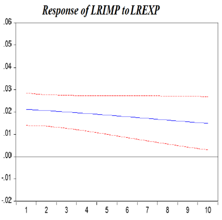
Figure 5 shows the generalized asymptotic impulse response function. It includes 16 small figures, which are denoted figure 5.1, figure 5.2, and so forth. Each small figure illustrates the dynamic response of each target variable (LRGDP, LREXP, LRIMP and LRFDIL) to a one-standard-deviation shock on itself and other variables. In each small figure, the horizontal axis presents ten quarters following the shock. The vertical axis measures the quarterly impact of the shock on each endogenous variable.
Figure 5.1 presents the long-run positive effect of a shock to LRGDP on LRGDP. This shock has a short- and long-run positive effect on LRGDP. Figure 5.2 shows that a shock to LREXP has no significant effect on LRGDP. Figure 5.3 shows that a shock on LRIMP has a negative effect on LRGDP. Figure 5.4 shows that a shock to LRFDIL has no significant effect on LRGDP. These effects do not conflict with the GCBEW test.


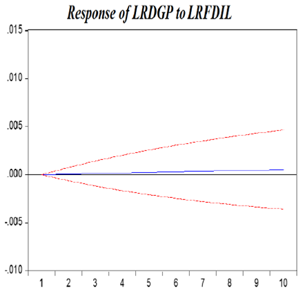
Figure 5.5 suggests that in the long run, a shock on LRGDP has a small significant positive effect on LREXP. Figure 5.6 suggests that LREXP has a positive effect on LREXP, as expected. Figure 5.7 shows a significant effect of LRIMP on LREXP and Figure 5.8 shows no significant effect of LRFDIL on LREXP. These results partly conflict with the GCBEW test, specifically with respect to the effect of LRGDP on LREXP.
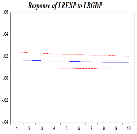


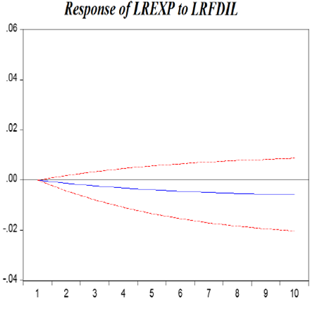
Figure 5.9 and 5.10 show the responses of LRIMP to shocks in LRGDP and LREXP; the shocks have a positive permanent significant effect on LRIMP. Figure 5.11 suggests that LRIMP has a positive effect on LRIMP, as expected. Figure 5.12 shows no significant effect of a shock in RDFIL on LRIMP. These results conflict with the GCBEW test, specifically with respect of the effect of LREXP on LRIMP.


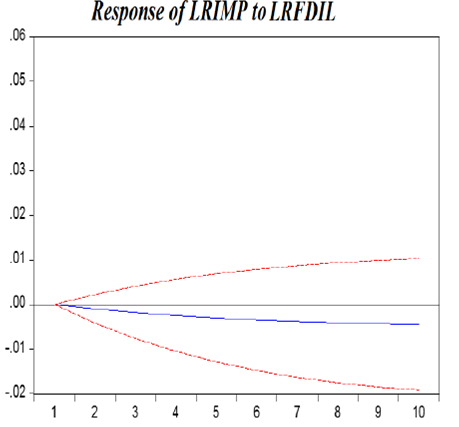
Finally looking at Figures 5.13 and 5.14 shows that a shock on LRGDP and LREXP has significant effect on RDFIL. The effect of shock on LRIMP has a negative effect on LRFDIL, as shown in Figure 5.15. Figure 5.16 suggests that LRFDIL has a positive effect on itself, as expected. These results do not conflict with the GCBEW test.


The Diagram 2, on the one hand, confirms the directions of causality that were offered in Diagram 1, according to the GCBEW test, as well as considering the positive effect of LRGDP on both LREXP and LRFDIL and the small, but negative, effect of LRGDP on LRIMP. In addition, we have a positive effect of LREXP on LRIMP and a positive effect of LRIMP on LREXP, which together show the inertia of international trade.

4.3. Variance decomposition
Variance decomposition (or forecast error variance decomposition) indicates the amount of information each variable contributes to the other variables in a VAR model (Enders, 2003). It tells us how much of a change in a variable is due to its own shock and how much due to shocks to other variables. In the short run most of the variation is due to a shock of its own, but as the effect of the lagged variables starts kicking in, the percentage of the effect of other shocks increases over time. Therefore, the variance decomposition defines the relative importance of each random shock in affecting the variables in the VAR. Table 10 includes 4 individual tables, one for each variable. The standard errors are given below the respective coefficient.
Table 10 Variance decomposition
| Period | S.E. | LRGDP | LREXP | LRIMP | LRFDIL |
|---|---|---|---|---|---|
| 1 | 0.0100 | 100.0000 | 0.0000 | 0.0000 | 0.0000 |
| 0.0000 | 0.0000 | 0.0000 | 0.0000 | ||
| 2 | 0.0141 | 99.5995 | 0.0000 | 0.3986 | 0.0018 |
| -0.4282 | -0.0553 | -0.4050 | -0.0593 | ||
| 3 | 0.0173 | 98.7705 | 0.0000 | 1.2234 | 0.0061 |
| -1.2156 | -0.1676 | -1.1529 | -0.1810 | ||
| 4 | 0.0201 | 97.6170 | 0.0001 | 2.3702 | 0.0127 |
| -2.1851 | -0.3215 | -2.0774 | -0.3492 | ||
| 5 | 0.0225 | 96.2265 | 0.0004 | 3.7515 | 0.0216 |
| -3.2209 | -0.5053 | -3.0683 | -0.5508 | ||
| 6 | 0.0248 | 94.6705 | 0.0012 | 5.2957 | 0.0326 |
| -4.2530 | -0.7100 | -4.0583 | -0.7753 | ||
| 7 | 0.0269 | 93.0061 | 0.0027 | 6.9457 | 0.0455 |
| -5.2420 | -0.9291 | -5.0092 | -1.0141 | ||
| 8 | 0.0289 | 91.2779 | 0.0052 | 8.6568 | 0.0601 |
| -6.1679 | -1.1583 | -5.9014 | -1.2605 | ||
| 9 | 0.0309 | 89.5203 | 0.0087 | 10.3947 | 0.0763 |
| -7.0227 | -1.3947 | -6.7263 | -1.5094 | ||
| 10 | 0.0327 | 87.7590 | 0.0134 | 12.1337 | 0.0939 |
| -7.8052 | -1.6364 | -7.4824 | -1.7570 | ||
| B: Variance decomposition of LREXP | |||||
| Period | S.E. | LRGDP | LREXP | LRIMP | LRFDIL |
| 1 | 0.04411 | 15.1124 | 84.8876 | 0.0000 | 0.0000 |
| -5.9917 | -5.9917 | 0.0000 | 0.0000 | ||
| 2 | 0.0608 | 15.6206 | 84.1512 | 0.1876 | 0.0407 |
| -6.0805 | -6.0452 | -0.3030 | -0.1514 | ||
| 3 | 0.07272 | 16.0900 | 83.1848 | 0.6002 | 0.1251 |
| -6.1641 | -6.0998 | -0.8719 | -0.4492 | ||
| 4 | 0.08215 | 16.5221 | 82.0277 | 1.2072 | 0.2430 |
| -6.2427 | -6.2147 | -1.5986 | -0.8437 | ||
| 5 | 0.08999 | 16.9198 | 80.7202 | 1.9747 | 0.3853 |
| -6.3161 | -6.4260 | -2.4142 | -1.2965 | ||
| 6 | 0.09672 | 17.2868 | 79.3013 | 2.8680 | 0.5439 |
| -6.3844 | -6.7438 | -3.2760 | -1.7790 | ||
| 7 | 0.10262 | 17.6270 | 77.8076 | 3.8533 | 0.7122 |
| -6.4488 | -7.1584 | -4.1574 | -2.2706 | ||
| 8 | 0.10788 | 17.9448 | 76.2714 | 4.8992 | 0.8846 |
| -6.5110 | -7.6484 | -5.0402 | -2.7569 | ||
| 9 | 0.11261 | 18.2446 | 74.7211 | 5.9776 | 1.0567 |
| -6.5730 | -8.1884 | -5.9101 | -3.2288 | ||
| 10 | 0.11691 | 18.5305 | 73.1803 | 7.0640 | 1.2251 |
| -6.6366 | -8.7541 | -6.75511 | -3.68054 | ||
| C: Variance decomposition of LRIMP | |||||
| Period | S.E. | LRGDP | LREXP | LRIMP | LRFDIL |
| 1 | 0.0463 | 5.9557 | 21.0369 | 73.0074 | 0.0000 |
| -4.8799 | -5.7367 | -6.6593 | 0.0000 | ||
| 2 | 0.0636 | 6.5252 | 21.7012 | 71.7510 | 0.0226 |
| -4.9124 | -5.8766 | -6.6356 | -0.1195 | ||
| 3 | 0.0759 | 7.0899 | 22.2494 | 70.5909 | 0.0699 |
| -4.9608 | -6.2784 | -7.0355 | -0.3662 | ||
| 4 | 0.0854 | 7.6483 | 22.6930 | 69.5223 | 0.1364 |
| -5.0218 | -6.8297 | -7.7025 | -0.7062 | ||
| 5 | 0.0933 | 8.1997 | 23.0439 | 68.5389 | 0.2175 |
| -5.0924 | -7.4455 | -8.4910 | -1.1084 | ||
| 6 | 0.0999 | 8.7437 | 23.3139 | 67.6337 | 0.3088 |
| -5.1697 | -8.0725 | -9.3027 | -1.5475 | ||
| 7 | 0.1055 | 9.2803 | 23.5139 | 66.7990 | 0.4068 |
| -5.2521 | -8.6812 | -10.0822 | -2.0037 | ||
| 8 | 0.1105 | 9.8098 | 23.6542 | 66.0275 | 0.5085 |
| -5.3384 | -9.2567 | -10.8021 | -2.4630 | ||
| 9 | 0.1149 | 10.3328 | 23.7439 | 65.3118 | 0.6115 |
| -5.4279 | -9.7921 | -11.4517 | -2.9151 | ||
| 10 | 0.1187 | 10.8498 | 23.7914 | 64.6450 | 0.7138 |
| -5.5204 | -10.2855 | -12.0292 | -3.3533 | ||
| D: Variance decomposition of LRIMP | |||||
| Period | S.E. | LRGDP | LREXP | LRIMP | LRFDIL |
| 1 | 0.1479 | 0.0034 | 1.1334 | 0.0409 | 98.8223 |
| -0.9559 | -2.0541 | -1.1617 | -2.6277 | ||
| 2 | 0.1997 | 0.0453 | 1.9660 | 1.1147 | 96.8741 |
| -0.9037 | -2.4161 | -1.5629 | -3.0759 | ||
| 3 | 0.2358 | 0.1534 | 2.8929 | 3.5426 | 93.4111 |
| -0.9159 | -2.7837 | -2.8537 | -4.1227 | ||
| 4 | 0.2646 | 0.3083 | 3.8340 | 6.7632 | 89.0945 |
| -0.9716 | -3.1786 | -4.3474 | -5.5358 | ||
| 5 | 0.2890 | 0.4918 | 4.7346 | 10.3160 | 84.4575 |
| -1.0506 | -3.6060 | -5.7983 | -7.0112 | ||
| 6 | 0.3103 | 0.6900 | 5.5641 | 13.8773 | 79.8685 |
| -1.1399 | -4.0569 | -7.0934 | -8.3536 | ||
| 7 | 0.3292 | 0.8931 | 6.3099 | 17.2482 | 75.5488 |
| -1.2325 | -4.5195 | -8.1948 | -9.4818 | ||
| 8 | 0.3460 | 1.0949 | 6.9704 | 20.3235 | 71.6113 |
| -1.3252 | -4.9851 | -9.1074 | -10.3845 | ||
| 9 | 0.3610 | 1.2916 | 7.5502 | 23.0610 | 68.0972 |
| -1.4168 | -5.4491 | -9.8554 | -11.0838 | ||
| 10 | 0.3743 | 1.4816 | 8.0570 | 25.4569 | 65.0046 |
| -1.5068 | -5.9089 | -10.4690 | -11.6131 | ||
Looking at Table 10-A, in the short run (that is, three quarters) a shock to LRGDP accounts for 98.77% of the fluctuation in LRGDP (own shock); a shock to LREXP can cause 0.00% fluctuation in LRGDP (not statistically significant). A shock to LRIMP can cause a 1.22% fluctuation in LRGDP (not statistically significant) and LRFDI a 0.01% fluctuation in LRGDP (not statistically significant).
In the long run (10 quarters), a shock to GDP accounts for 87.76% of fluctuation in LRGDP, LREXP for 0.134% (not statistically significant), LRIMP 12.13% (statistically significant) and LRFDIL for 0.09% (not statistically significant). Therefore, in the short run, none of the variables have a statistically significant effect on LRGDP, and in the long run, only LRIMP does.
Looking at Table 10-B, in the short run, a shock to LREXP accounts for a 83.18% fluctuation in LREXP (own shock), a shock to LRGDP causes a 16.09% fluctuation in LREXP (statistically significant). A shock to LRIMP causes a 0.60% fluctuation in LREXP (not statistically significant) and LRFIL a 0.13% fluctuation in LREXP (not statistically significant).
In the long run, a shock to LREXP accounts for 73.18%, LRGDP to 18.53% (statistically significant), LRIMP 7.06% (not statistically significant) and LRFDIL 1.23% (not statistically significant). Therefore, in the short and long run, only LRGDP has a statistically important effect on LREXP.
Table 10-C shows that in the short run a shock to LRIMP accounts for 70.59% fluctuation in LRIMP (own shock), a shock to LRGDP can cause 7.09% fluctuation in LRIMP (statistically significant). A shock to LREXP can cause 22.25% fluctuation in LRIMP (statistically significant) and LRFIL a 0.07% fluctuation in LRIMP (not statistically significant).
In the long run, a shock to LRIMP accounts for 64.65%, LRGDP to 10.85% (statistically significant), LREXP 23.79% (statistically significant) and LRFDIL 0.71% (not statistically significant). Therefore, in the short and long run, only LRGDP and LREXP have a statistically important effect on LRIMP.
Looking at Table 10-D, in the short run, a shock to LRFDIL accounts for 93.41% fluctuation in LRFDIL (own shock). A shock to LRGDP can cause 0.15% fluctuation in LRFDIL (not statistically significant); a shock to LREXP can cause 2.89% fluctuation in LRFDIL (not statistically significant) and LRIMP a 3.54% fluctuation in LRFDIL (not statistically significant. In the long run, a shock to LRFDIL accounts for 64.00%, LRGDP to 1.48% (not statistically significant), LREXP 8.06% (not statistically significant) and LRIMP 25.46% (statistically significant). Therefore, in the short run, none of the variables have a statistically significant effect on LRFDIL, and in the long run, only LRIMP has a statistically important effect on it.
From the GCBEW test, the impulse-response analysis and the variance decomposition analysis, we can conclude the following:
All three indicate that FDI has no effect on GDP growth or international trade.
All three indicate the existence of bidirectional effects between imports and GDP and of a unidirectional effect of imports on FDI (although the sign is contradictory).
Impulse-response analysis and variance decomposition coincide in showing that GDP growth has a positive effect on exports.
GCBEW test and the variance decomposition analysis establish postive effects of exports and GDP on FDI.
We find no evidence of the exportled growth hypothesis.
4.4. Lessons for Mexico
The causal dynamics of foreign trade and investment magnitudes with respect to economic growth are a particularly important topic for investigation; especially in the case of Korea, which has often been taken as an example to emulate due to the outstanding growth rates of its economy in the last decades. Accepting the exports-led growth hypothesis for Korea would not be, necessarily, a justification for its implementation in Mexico, because, as we have seen, the effects of trade on the rest of the economy may vary among countries, depending on their initial conditions and the strength of their institutions. However, our findings show that, in the representative case of Korea, economic growth responded to an internal logic and not to the increase of exports.
From the 1980s, Mexico began a period of export substitution, during which manufacturing exports began to have a greater relative importance than oil (Villarreal, 2005). In parallel, the 1980s meant a decade of increased FDI for Mexico. The opening of the Mexican economy to international competition has been intense since the signing of NAFTA in 1994. However, none of these policies have led to high levels of economic growth for Mexico.
The final objective of export promotion policies should not be simply to increase exports, but rather, to achieve higher economic growth rates. The mere opening of a country does not guarantee the creation of a productive sector: productive abilities are created internally. Thus, despite the importance of the external sector, as, for instance, a signaling mechanism for those firms to improve their competitiveness; policy makers should not just focus on an increase of exports. As we have seen, even in the case of Korea, we must be cautious about the effect of exports on economic growth.
We should properly understand the developmental models that Mexican policy makers take as a reference. If, as is claimed in this paper, it is the case that exports and FDI are not the causes of Korean economic growth, we should consider possibly reorienting the Mexican growth model. Instead of focusing on further boosting a very concentrated and highly productive external sector, policy makers should consider the adoption of an industrial policy that creates production capabilities within the country, regardless of whether such production is exported. Exports will come as a consequence of this improvement.
5. Conclusions
In this paper, we have made an empirical analysis of the economic growth in Korea between 1980 and 2015, in order to identify the potential relationships between relevant variables. In doing so, we have implemented a methodology similar to Nguyen (2011). Our econometric procedures include the unit root test of relevant series, lag structure, the VAR diagnostic, the Johansen cointegration test, the Granger causality/Block exogeneity Wald test (GCBEW), an analysis of impulse response and analysis of variance decomposition. One of the main results of this paper is that, for the Korean case, GDP growth cannot be explained by increased exports. We believe that this is an important result, since it not only confronts the export-led growth hypothesis for the Korean case, but also undermines the export promotion agenda as a tool to promote Mexicos development.
The advantages of trade liberalization for economic growth and development have been broadly debated in the relevant literature. Up until the mid-1970s, import substitution policies prevailed in most developing countries. Since then the emphasis has shifted towards export promotion strategies in an effort to promote economic development. It was hoped that export expansion would lead to better resource allocation, creating economies of scale and production efficiency through technological development, capital formation and employment generation. The shift also included an increasing reliance on FDI. The results of imposing and implementing those policies in Latin America, Africa and some East European countries have been disappointing.
The realities of Korea’s successful growth case teach us a lesson and suggest that we may have to unlearn some lessons that we have been taught, and that we need to reconsider the effectiveness of the traditional laissez-faire approach as a tool to boost economic development. As the Korean experience shows, growth in exports and a liberal trade policy cannot be seen as silver bullets that promote development, but rather as parts of a complex mechanism that may well expand the benefits of a whole set of policies that push the industrialization and economic growth of a country. These are the benefits that have been denied to Latin America by the multinational institutions and economic orthodoxy that have dominated the region for more than three decades.

