nueva página del texto (beta)
 Inglés (pdf)
 Artículo en XML
 Referencias del artículo
 Enviar artículo por email
 Citado por SciELO
  Similares en
SciELO
Similares en
SciELO 
 Permalink
1. Introduction
Monitoring and improving the fiscal system is a relevant issue for developing countries for three main reasons: 1) This mechanism represents the most efficient and effective tool for improving the distribution of wealth, by making it possible for taxes to be more progressive; 2) Tax evasion in developing countries has become practically the rule, due to the growing size of the informal sector, underlining the need for improving the fiscal system; 3) The impact of government benefits on the poor via transfers and social programs decreased across Guatemala and México over the nineties according to Gomez (2006), and Heston, Summers, and Aten (2006), increasing the need for progressive fiscal systems. In any case, we emphasize the inequality concept as a benchmark for understanding and quantifying levels of progressivity in the process of acting of the tax system itself.
Over the past 15 years, Latin American countries with a similar level of development as Mexico, such as Brazil, Argentina and Uruguay, have shown greater improvement in the degree of progressivity of their fiscal systems, and have obtained greater redistributive effects (Lustig, Pessino, and Scott, 2014). Furthermore, in comparison with Mexico’s Oportunidades program, several poorer economies, such as Bolivia and Peru, have obtained better results in fighting poverty, having applied programs that were even more ambitious and were supported by fewer resources (Araar, 2012).
In this paper, we study the evolution of the degree of progressivity of Mexico’s tax-benefit system from 2002 to 2012. This retrospective form of analysis is helpful to provide some salient facts about the relevance of the fiscal policies and social programs that were implemented during this period. We also attempt to provide a thorough analysis of the problems associated with comparing the degree of progressivity of a fiscal system over time, an approach that has been absent in the empirical literature. We do this by providing a common support for comparison of temporal changes in the distribution of gross income.1
Our method can be generalized, and applied to other cases, for instance, to compare degrees of progressivity across countries. Empirical research has been carried out before to measure the tax burden or even the incidence of transfers and benefits over time and across countries. For example, the research of Kniesner and Ziliak (2002) examines the effect of the federal income tax reforms of the 1980s in the United States on the degree of automatic stabilization of consumption. They determined that the social program reforms implemented during this period increased the degree of automatic stabilization, whereas tax reforms, including The Economic Recovery Tax Act of 1981 (ERTA) and the Tax Reform Act of 1986 (TRA86), reduced consumption stability by about 50 percent for households at risk for large fluctuations in income, and that the impact were much more modest for the typical household.
In our research, we decided to focus on the period from 2002 to 2012, because in 2002, an opposition party (the Partido Acción Nacional, PAN) won the elections for the first time in seventy years, and remained at the helm over this period. Indeed, some important changes took place during these 12 years. At the state/local level, the tax systems remained weak and the informal sector grew up to reach sixty percent of the workers by the end of the period (INEGI, 2014), resulting in a low taxable base. In addition, the benefit programs began to grow faster during this period. These facts can provide an ideal opportunity to examine the temporal effects of the fiscal policy and redistribution into the whole population as well as for the contributors.
Another interesting feature of this period is that it provides us with an opportunity to study the response of the tax-benefit system to the 2008/2009 international financial crisis. One of the main salient facts of this crisis was the rapid increase in internal food and energy prices. This led to an expansion of consumption subsidies and targeted benefits, as well as to an increase in the value-added tax (VAT), from 15 to 16 percent, except for the six states bordering those of the United States of America (US) where the increase was from 11 to 16 percent.
The rest of the paper is organized as follows. The next section describes briefly the international fiscal context and its main effects on some developed and undeveloped countries, and explains the main features of the Mexican fiscal system from 2002 to 2012. The third section describes the theoretical framework. The fourth presents the data sources, specific assumptions and the empirical exercise. Section five concludes and provides some final insights, providing new routes for future research.
2. The tax-benefit system behavior in perspective
The tax-burden in Latin America is low in comparison to other countries with similar levels of economic development, averaging 15 percent in 2005. However, differences among countries remain large, with the tax burden ranging from about 35 percent in Brazil to as low as 10 percent in Mexico and Guatemala. The trend during the last decade has been towards increasing the tax burden and improving its efficiency, particularly in countries such as Argentina, Chile Bolivia and Peru that started the period with similar patterns of low efficiency in the collecting of tax revenues. Public expenditure levels, in contrast, have differed widely among the Latin American economies during the last twenty years, and this difference has been increasing since 2002.2
In Canada, Davidson and Duclos (1997) found an increasingly progressive fiscal system in the post-fiscal distribution of income between 1981 and 1990. Using the asymptotic sampling distribution of quintile-based estimators, they found that taxation is clearly statistically less progressive than an equivalent amount of government benefits, and that gross incomes were more equal in 1981 than in 1990; the opposite trend was found for net incomes, i.e., redistribution was significantly more progressive in 1990 than in 1981.
Wagstaff and van Doorslaer (2001) analyzed the role of tax credits, rate structures, allowances and deductions, in order to determine the overall progressivity of net income tax liabilities in fifteen OECD countries, and they found three kinds of clusters. First, they found that the dominant (but not only) effect driving progressivity of gross and net tax liabilities in countries like Australia, France, Italy, the Netherlands and Spain is the rate structure. Second, they found a group of countries where available allowances and transfers are the dominant source of progressivity, as is the case in many Englishspeaking countries. Finally, they found a third group of countries characterized by a mixed structure, including Belgium, Finland, Germany and Sweden, where roughly half of the progressivity of gross tax liabilities is attributable to the rate structure, and the other half to allowances and transfers.
In a more recent study on Canada, Araar (2008) performed an empirical application for progressivity to estimate the impact of the fiscal system on the size and wellbeing of socio-economic classes. He concludes that the progressivity of the fiscal system enabled a reduction in the number of the poor and an increase the size of the middle class, between 1993 and 2005.
On the other hand, tax progressivity may increase inequality, especially in countries having a weak legal system and a large informal nontaxable sector. Duncan (2010) found such a pattern for over one hundred countries worldwide, and suggests that progressivity increases inequality in reported gross and net income, with this effect being much stronger in countries whose institutional framework supports a pro-poor redistribution. A similar pattern was found in Claus, Martinez-Vazquez, and Vulovic (2013) for many Asian countries.
Baunsgaard and Symansky (2009) highlight reasons why analyzing income taxes is important, including the relative progressivity of income taxes relative to corporate or consumption taxes over time. For example, corporate taxes do not act as significant automatic stabilizers in the economic cycle (Devereux and Fuest, 2009, and Buettner and Fuest, 2010). Also, Attinasi, Checherita-Westphal, and Rieth (2011), using a direct measure of personal income tax progressivity, found that personal income taxes seem to be more important in terms of budgetary revenues than corporate income taxes for many developed EU economies. They show OECD cross-country evidence on the relationship between tax progressivity and output volatility.
For the Latin American case, Lustig, Pessino, and Scott (2014) provide good insights on the effects of the degree of fiscal progressivity in six countries in the region, and its impact on poverty during 2000-2010. Their findings show a more progressive tax-benefit system for most of the selected countries in recent years, although there are major cross-country differences. The fiscal systems of Bolivia, Mexico and Peru have the lowest impacts on poverty reduction, while Argentina, Uruguay and Brazil presented the greatest reductions in poverty, as well as being the countries with the most redistributive fiscal systems.
Precisely, for the Mexican case included in the same special journal issue, Scott (2014) presents a complete analysis of its fiscal taxbenefit system for a short period: between 2008 and 2010. Scott finds that the fiscal system is trapped in which he calls a “low-revenuelow-benefit equilibrium”, where low tax revenues are not the result of exceptionally low tax rates, but instead result from low levels of tax productivity. His findings show a more progressive fiscal system in 2010 than in 2008.
Although Lustig, Pessino, and Scott (2014) and Scott (2014) have done a great job in processing the tax figures and transfers in their databases, their findings with regard to progressivity could be biased because a formal common support of comparison was not used in their estimations over time. In order to estimate a comparable set of inequality and progressivity indices across the years, the initial or the final conditions of income distribution must be used.
2.1. Overview of changes in the Mexican fiscal structure
Serious distortions that result in an excess of inequality persist among the population in Mexico, both in how they pay taxes as well as in the way the poor receive welfare support through the fiscal system. While inequities in Mexico have historical roots, a better redistribution of resources can be achieved through the fiscal systems, using compensation-based redistributive policies, which work not only in developed but also in developing countries.
Two other issues of importance in Mexico are the significant underreporting of wages by registered firms to evade payroll taxes in the country (Kumler, Verhoogen, and Frias, 2013), as well as the impact of a persistently high level of employment in the informal sector with serious consequences for the marginal efficiency of taxation. The informal sector accounted for between 45 and 80 percent of total employment in Mexico between 2005 and 2010 (Dougherty and Escobar, 2013). Both of these factors contribute to the persistently low levels of revenue collection. It is possible that the latter will cause the tax system, even when it is progressive, to be unable to significantly affect inequality over time.
It is important to remark that the taxation structure remained virtually unchanged in Mexico from 2004 to 2012, and that the main taxation figures show relatively few changes. Income taxes remained the same at the margin, although the VAT changed in 2010, increasing the general rate from 15 to 16 percent, leaving the rest of consumption categories unchanged. Income taxes accounted for an average of 46 percent of total taxation revenues, and VAT 38 percent, during the period.
Two direct taxes were introduced in 2008. The first was the business flat tax (IETU for its initials in Spanish), with a minimum threshold of 17.5 percent. This flat tax had a broader basis than the income tax (both personal and corporate), and it was levied on agents who paid no income tax, making taxation more equitable and reducing fiscal evasion. The second tax was the flat tax on cash deposits (IDE in Spanish), with a flat rate of 2 percent applied to cash deposits in the banks that exceeded 15 000 Mexican pesos per month. This tax was supposed to be paid by all agents in order to reduce informality as well as to cope with organized crime. These taxes were eliminated in 2013 and accounted for no more than 4.1 and 1.3 percent of total taxation revenues respectively in 2011.
This structural fiscal crisis, which has characterized the Mexican government for decades, highlights the need to better target public expenditures towards vulnerable sectors of the population. The economic policy of the last two decades, which was aimed mainly at maintaining macroeconomic balances, produced neither higher economic growth nor the consolidation towards a more equitable society. On the contrary, deterioration in the living conditions of the Mexican society is evident: in 2012 more than 50 percent of the population lived below the official poverty threshold, compared with 42.6 percent in in 2006, the minimum level over the period examined.3
Is it possible to improve the social efficiency of benefits, as well as the tax efficiency, in order to increase financing for social programs as well as for public projects in this country? The need for continued improvements in the design of a tax-benefit system is justified by structural changes in the Mexican economy. For instance, an increase in the tax-burden on the production or consumption of goods may be relevant in order to compensate taxpayers, particularly when the informal sector comes to dominate the economic structure (Dougherty and Escobar, 2013).
Other social transfers such as aid to the elderly or, for areas with natural disasters or with serious problems in the creation of jobs, and additional aid accompanied the well-known social assistance program Oportunidades created in the year 2002, in the form of food assistance for the poor. These programs have not been very efficient at reducing poverty during this period of analysis, accounting for no more than 0.92 percent of Mexican Gross Domestic Product (GDP) at most, in 2010, and were accompanied by an equal increase in average poverty gaps for the Mexican households.4
2.2. Growth and shocks: An inability to finance public spending via taxes
Among Latin American countries, Mexico has the lowest level of efficiency of its fiscal system and the lowest level of public spending as a share of GDP. Data from Heston, Summers, and Aten (2006) signals Colombia and Brazil as the countries with the highest levels of public spending as a share of GDP in 2005 (28.3 and 22.4 percent respectively); followed by Costa Rica, Peru and Paraguay (15.6, 15.7 and 16.8 percent correspondingly); with Mexico in last place, with 13.3 percent.
World Bank (2014) information reveals that the Mexican economy has struggled recently with two years of crises: 2001 and 2009. These years saw a deceleration of GDP growth, by -1.55 and -7.1 percent, respectively. The period 2001-2009 shows evidence of a shift of employed workers from manufacturing to services. Caamal (2013) shows this pattern to be associated with lower labor demand in the former sector and falling returns to education. Government actions during this period centered on two important features: Application of a generalized consumer subsidy on domestic electricity, gas and diesel, as well as gasoline; and an increase from 0.34 to 0.92 percent of GDP in the direct cash-transfer social programs. The consumer subsidies have varied sharply in recent years as a function of international oil prices: they accounted for a historical maximum of 2.8 percent of GDP in 2008. Domestic gasoline prices rose gradually during the first decade, while international gasoline prices rose, and then domestic gasoline prices increased by 0.11 Mexican cents every month. Afterwards, Mexican fiscal authorities kept a fixed rate of increase for internal sales of gasoline and kept revenues at about the same level of GDP until 2014, when international prices of oil dropped drastically.5
During 2006-2012, the government introduced a non-contributory health insurance program, Seguro Popular, to cover most of the uninsured population, mostly the poor.6 People who had neither coverage of social security, nor any protection from a health care program (public or private) could apply for it. Under this program, the number of uninsured people decreased from 50.1 percent of this group (13.3 million individuals) in 2006 to 44.1 percent (11.8 million individuals) in 2008. Between 2008 and 2012, the overall number of uninsured decreased significantly to 21.5 percent (25.3 million people), according to Coneval (2014). This significant decrease is mainly due to the enrollment in the Seguro Popular system.
According to Scott (2014) these subsidies and programs have been implemented despite a failure to improve Mexico’s low efficiency of revenue mobilization. Non-oil tax revenues have remained stagnant at less than 10 percent of GDP, while the rest of the Latin American countries have seen revenues rise on average by 13 to 19 percent of GDP in the last ten years. As a result, a large fraction of Mexico’s public spending is financed through oil revenues that come from the state-owned oil company Petróleos Mexicanos (PEMEX).
Campos, Esquivel, and Lustig (2012) studied disposable total household income in Mexico, and found that inequality decreased from 2002-2006 and then returned to its 2002 level in 2008, with a standard Gini coefficient of 0.51. Inequality then decreased to 0.49 in 2010. Among the factors driving this process, they identify the decline in non-labor income inequality and the role exerted by remittances and government transfers. From 2002 to 2010, emigration from Mexico to the US grew at a rapid pace, as did remittances sent by these migrants to their families in Mexico. Coneval (2009) data provides evidence that without remittances, poverty figures in the country could have been much higher.
3. Theoretical framework
In this section, our main objective is to present the theoretical framework used in this study by focusing on how we: 1) assessed the progressivity of a fiscal/benefit system; 2) developed a comparison of progressivity over time, and 3) assessed the distributive impact of the fiscal/benefit system.
We start by introducing the theoretical framework we used to test and measure the progressivity of taxes or benefits. Then, we explain the inequality and polarization indices used to assess the behavior in income disparities and the polarization of income arising from the tax-benefit redistribution.
3.1. Testing the progressivity of the fiscal system
Usually in distributive analysis, we assess the progressivity of taxes or transfers. However, governmental intervention through the fiscal system will have either a negative or a positive impact on the gross income of a household, depending on its characteristics. First, we begin by dividing the total impact of the fiscal system on household income, which is the difference between net and gross income, into two main components. If the household-level impact is negative, we assume that the latter represents a global tax, noted by T, that the household must pay. In contrast, if the impact is positive, this represents a global transfer that the household receives and we denote it by B. It can be said that a tax is progressive if the tax burden of the poor group is relatively lower than that of the non-poor group. This implies a rise in the share of net income for the poor group. In the literature of progressivity, there are two main distinct concepts of progressivity, which are local progressivity and global progressivity. Musgrave and Thin (1948), in their pioneering work, proposed two main approaches for the measurement of local progressivity: liability progression (LP) and residual progression (RP). Let V (x) denote the final impact on gross income x, such that V (x) = B(x) − T (x).
THEOREM 1. With the liability progression measurement, a fiscal system with tax T and transfer B is locally progressive if and only if:
where ηT and ηB refer to the elasticities with respect to income x for tax T and transfer B, respectively.
PROOF. The liability progression condition of the net benefit V(x) = B(x)−T(x) can be derived starting from that of the local progressivity at x: η (V(x)) < 1. Thus, we can write
After rearranging this condition, we find that:
or also
Finally, one can define the liability progression curve (LP (x)), which can be used to test liability progression at different levels of income:
Note that that with the residual progression measurement, a fiscal system with tax T and transfer B is locally progressive if and only if:
RP(x) = η N (x) ˂ 1 (6)
where η N (x) refers to the elasticity of net income N (x) with respect to income x.
To test the global progressivity of a fiscal system, we use two approaches. The first is the Tax Redistribution approach (TR), which is based on the distribution of taxes with respect to gross income. The second is the Income Redistribution approach (IR), which is based on the distribution of net income as a function of gross income.
THEOREM 2. A fiscal system with tax T and transfer B is globally TR progressive if and only if:
Where L x (p) and C x (p) denote the Lorenz and concentration curves respectively at percentile p, and where μT and μB are the average tax and average transfer respectively.
PROOF. For an individual i with gross income x i , we denote the impact of the fiscal system by z(x i ) such that:
z(x i ) = f B (x i ) - f T (x i ) + K i (8)
Of course, when the fiscal system is progressive, the impact should decrease with the increase of income (i.e. z'(x) < Ɐ x For a deterministic function of the impact, the random component (κi) must be nil. In this case, the local liability progression at x requires that f' B (x) > f' T (x). As is well known, the ultimate objective of making the tax progressive is to reduce inequality. However, the question is: to what form of inequality we refer? The Atkinson (1970) theorem makes it possible to check for a reduction in inequality measured by a class of indices that obey the basic axiom of inequality: the Dalton transfer principle. More precisely, the Atkinson theorem stipulates that if the Lorenz curve of the post fiscal distribution is everywhere above that of the pre-fiscal distribution, then all inequality indices that obey the Dalton transfer principle will decrease. In the absence of re-ranking, the concentration curve becomes a helpful tool to test for the progressivity of a tax system. Starting from the Atkinson condition, we can write:
Thus, the condition becomes:
Since the ratio
Finally, we find that the condition can be simplified as follows:
It can be easily checked that if TR(p) is greater than zero across the entire range of percentiles, and in absence of re-ranking, then the redistributive effect of this fiscal system is socially efficient and inequality must decrease.7 Instead of comparing Lorenz and concentration curves, we can use progressivity indices. The aim of these indices is to capture progressivity across the entire income distribution with one summary index. In general, these indices are computed as differences between the Gini and concentration indices.8
COROLLARY 1. A fiscal system with tax T and transfer B is progressive if the index of progressivity:
where IG and IC are the Gini and concentration indices respectively. For the IR approach, it can be said that the fiscal system is IR progressive if:
Using Gini and concentration indices, we can corroborate that the fiscal system is progressive if:
3.2. Comparison of progressivity over time
As stated above, it is not possible to directly compare the estimated progressivity indices in order to assess the nature of change in the progressivity of fiscal systems over time, because the distribution of gross income varies from one year to another, which raises the problem of the absence of a common support of comparison. In fact, changes in the pre-tax income distribution substantially affect progressivity measures, even with an un changed fiscal system.9 The less equal the gross income distribution, the greater the equalizing effects and hence, the higher the progressivity index. Hence, progressivity indices cannot be compared with the change in the distribution of gross income over time.10
To address this issue, we propose to compare progressivity indices or curves, when the reference year is predetermined. For instance, to compare the progressivity of a tax-benefit system between periods 1 and 2, and when the reference period is period 1, the expected taxes and transfers from period 2 can be estimated using information (incomes, taxes and transfers) from period 1. For analytical purposes, we generally focus on the most updated distribution of wellbeing and we try to show whether there is an improvement in the progressivity of the tax-benefit system over time.
Formally, let
3.3. Inequality and polarization
In this study, we use the popular Gini index to assess the levels of inequality in gross and net incomes. This enables us to show by how much the tax-benefit system reduces income disparities. Also, we assess the impact of the tax-benefit system on polarization, measured by the Foster and Wolfson (1992) (FW) and Duclos, Esteban and Ray (2004) (DER) indices to assess bipolarization and polarization respectively. Formally, the normalized DER index can be written as follows:
Where A = 0.5µα-1 and f (.) is the density function and x and y stand for gross and net incomes respectively. Keep in mind that when the parameter α = 0 the normalized DER index equals the usual Gini index. The question that can now be raised is: How do polarization indices differ from those of inequality? While inequality measurements are used to assess the expected divergence or disparity between incomes, polarization measurements are also sensitive to the level(s) of income used to classify the income groups. For a given population group delimited by a small income range, its identification increases with its population share.11 Furthermore, it has been argued that there is a clear link between polarization and some other negative aspects of the distribution. For instance, severe poverty, disappearance of the middle class or a higher level of between-group inequality are certainly related to the phenomena of polarization.
Next, we review the bipolarization measurement adopted in this paper. Bipolarization (FW) can be viewed as a special case of polarization, focusing on the level of disparity and on identifying the two main population groups. For the FW index, the first group is composed of those with incomes below the median and the second includes those with incomes above this threshold. Rodríguez (2004) proposed an interesting representation of this index:
Where IGB m and IGW m are the between and within inequality components, when the Gini index is decomposed by the two population groups (one group with incomes below the median income (m), and the other with incomes above this level). Hence, the FW index reaches its maximum when the first half of the population has a null income and the second half equally shares the entire total income. In general, any distributive change that increases the average income of the rich group will increase bipolarization measurements. In addition, a decrease in inequality within any of these two groups will increase the degree of bipolarization (groups will be more identified through income). In summary, this index gives us synthesized information about the level of disparity in average income between the two main groups of the population and how homogeneous the income levels of these two sets are.
4. Empirical application
4.1. The Mexican household income and expenditure surveys
For the empirical exercise, we unified a series of microdata from the survey Encuesta nacional de ingreso y gasto de los hogares (ENIGH) carried out by Instituto Nacional de Estadística y Geografía (INEGI, 2013) using data from the years 2002, 2004, 2006, 2008, 2010 and 2012. Incomes are deflated using a CPI with 2012 as a reference year; the surveys were carried out in the month of August. Based on the information provided by the microdata, we proceed to build the distribution according to the Coneval (Consejo Nacional de Evaluación de la Política Social) equivalence scale and followed both direct and indirect identification methods, in order to make it comparable to the official reports.12 See Appendix 1 for a brief explanation of the construction of the fiscal system.13
In order to ensure an accurate estimation of wellbeing for household members, we use the individual as the main unit of distributive analysis, and since there is a consensus on the relevance of such an approach. In our case, we use the equivalence scale from Coneval (2009) to account for individual wellbeing. The adult equivalent scales are defined as follows (age ranges in brackets): [0-5]=0.7, [6-12]= 0.74, [13-18]= 0.71, and [19-65+]= 0.99. In this sense, we are comparing homogeneous units with respect to the level of income necessary to meet their needs.14 Also, we use a micro-accounting approach where behavior at the micro (survey) level is not considered. This is not a problem in our case, as has been shown in Pudney and Sutherland (1994) and Bourguignon, Bussolo, and Pereira (2008). Those studies prove that the relevant issue is the robustness achieved in relative terms from the action of the fiscal system with respect to income distribution, regardless of any the under-reporting of income presented (or taxes paid) in the top part, as long as the calibration of data is sufficiently representative, which is the case in our analysis. It is worth noting that the task of analyzing the tax effects on poverty goes beyond the scope of this research.
It can be seen in Figure 1 that, during the 2002-2012 period, income tax reforms have been modest. Thus, we cannot expect the reforms to significantly impact government revenues. As we can observe in Figure 1, for people in the highest income bracket, the maximum rate of 33 percent in 2004 decreased to 28 percent in 2008 and rose to 30 percent in 2010. However, when real brackets are considered using 2012 as the base year, it can be seen in Figure 2 that for middle-income earners (above 30 000 monthly pesos) the tax burden increased over this period. Although, the marginal tax rate for middle and top earners, in nominal units, seems to have reached its highest point over this period in 2004; when correcting for inflation, it becomes clear that the top marginal tax rate was reached in 2012. Following the tax changes in 2010, the tax burden for middle-income earners in 2012 was higher than in 2004 and 2008. Tax reform not only led to a higher marginal tax in 2012 (33 percent) than in 2004 (30 percent), but it also widened the brackets for the middle and the top earners, which diminishes the likelihood of falling into the next lower bracket when faced with an exogenous drop in income.

Source: Authors' elaboration using data from the Mexican Ministry of Finance, SHCP, 2014 and ENIGH, 2004, 2008 and 2012 databases.
Figure 2
The adjusted data also shows that the real tax burden increased disproportionally for the low-income earners (less than 10 thousand pesos), in 2012, perhaps due to relative price changes in taxable goods consumed most intensively by the poor. This resulted in decreased welfare for these contributors to the fiscal system and offset the progressivity of the fiscal system in general.15
This situation was compensated by the addition of cash benefits to gross incomes, as we will see in the empirical application section. The comparison in the previous paragraph is the result of compensating for inflation in the period, which is captured by the CPI index when brackets are deflated. It makes sense that the progressivity of gross tax liabilities could be caused by the income tax rate structure, but further research would be necessary to confirm this.
4.2. Composition of population and household wellbeing
A useful method for obtaining a complete picture of the shape of the distribution of wealth is to draw its density function. For this purpose, we have selected three years of surveys in the period (2004, 2008 and 2012), and estimated the density functions using the Gaussian corrected boundary kernel estimator. The usual kernel estimation will be biased when close to the minimum bound. In our data the corrected boundary kernel estimator was needed due to the high frequency of the population with low or no market income.
In Figures 3 and 4, we plot density functions of gross and net income respectively. Two changes are worth pointing out. First, the shift of the density curve of net income to the right between 2004 and 2012 indicates that household wellbeing increased on average during this period, although in 2008, the density curve moved to the left, marking the negative impact of the world economic shock of 2007/2008. Second, the shape of the density function of gross income flattened over this period. Recall here that inequality is inversely linked to the kurtosis of the distribution.16 Thus, for flatter density functions, the population size of the poor and rich groups is relatively greater, indicating a higher than expected disparity in income or inequality.

Source: Authors’ elaboration using ENIGH, 2004, 2008 and 2012 data.
Figure 4 Density curves of net incomes
Next, we examine the main factors that explain the change in average income during the period studied. In figure 5 we start by presenting the trend of some basic macroeconomic indicators. Among the important points, we can see the clear negative impact of the world economic shock of 2007/2008 on the Mexican real gross domestic product. The inflation rate remained practically constant, but food prices did not; also, the unemployment rate registered an increase during the world economic crisis. Note that even in the case of constant returns in endowments (real wage for instance), the change in the composition of the population, expressed by the change in the proportion of the working age population, may cause a variation in average income. The trend of real GDP plotted in Figure 5, indicates that substantial economic improvement arrived at the end of the period studied, following a 7.1 percent decline in production in 2009. However, the active population rate showed an increase.
Source: Authors’ calculation using ENIGH data from the corresponding years.
Figure 5 The trend of Mexican macro-economic indicators
This conclusion is also confirmed in Figure 6, which shows that the expected household size for a given level of gross income has decreased over time. This increase in welfare through the change in the composition of the population, or equivalently, this decrease in the ratio of dependence, may be temporary. The renewal of the active population must be perceived as an inter-generational investment, necessary for ensuring the availability of an adequately-sized active population in the long term. While the proportion of children in the population was about 45.87 percent in 1960, the proportion decreased to about 29 percent in 2012. It may be helpful to look for demographic policies to remedy this decline, and to examine how fiscal policy should change in response.
4.3. The trend of inequality and polarization
As reported in the Theoretical framework section, inequality indices are useful for summarizing information on disparities in personal incomes. In Table 1, we present the trend of inequality in gross and net incomes for the period between 2002 and 2012. The following remarks summarize the important points:
There has been a slight decrease in inequality between 2002 and 2012 for both gross and net incomes. However, this decrease was much larger just after the world economic shock of 2008. Araar (2012) reports how inequality and poverty for some Andean (specifically Bolivia and Peru) as well as other Latin American countries decreased just after the world economic shock of 2007/2008. His work, which did not examine Mexico, ascribes falling inequality to the large impact on targeted beneficiaries of the social programs.
The impact of the fiscal system seems to be positive, and depends mainly on the shape of the distribution of gross income. This conclusion is based, in part, on the stable impact of the fiscal system on inequality, but only for each year: the effect is not cumulative, so its impact disappears and inequality returns to its initial level of inequality. This may be due to the rigidity of adjustment of the fiscal system over time, or to its delay in responding to economic shocks. The fiscal system accounts for only about 6 points of the yearly reduction in the Gini index (column 3 of Table 1).
Table 1 The trend of inequality in Mexico
| Gross income | Net income | Change (%) | Gross income | Net income | Change (%) | |
| 2002 | 0.559 | 0.520 | -0.070 | 0.025 | 0.024 | -0.035 |
| 2004 | 0.545 | 0.508 | -0.066 | 0.025 | 0.024 | -0.028 |
| 2006 | 0.542 | 0.509 | -0.061 | 0.014 | 0.014 | 0.048 |
| 2008 | 0.556 | 0.522 | -0.060 | 0.018 | 0.018 | -0.044 |
| 2010 | 0.530 | 0.494 | -0.068 | 0.007 | 0.008 | 0.117 |
| 2012 | 0.548 | 0.513 | -0.064 | 0.015 | 0.016 | 0.037 |
Source: Authors’ calculation using ENIGH data from the corresponding years.
Over time, there has been a substantial decrease in inter-regional inequality when we compare those in the northern border zone and the rest of the country. However, it is not clear that fiscal policy played a part in this decline.
Next, we focus on the evolution of polarization in Mexico and how governmental interventions, through taxes and transfers, have reduced its level. In Table 2, we present the trend of the DER polarization index from expression (17) for gross and net incomes.
Table 2 The trend of polarization in Mexico
| Year | DER index (α=0.75) | FX index | ||||
| Gross income | Net income | Change (%) | Gross income | Net income | Change (%) | |
| 2002 | 0.267 | 0.251 | -0.059 | 0.522 | 0.463 | -0.113 |
| 2004 | 0.258 | 0.244 | -0.055 | 0.496 | 0.451 | -0.090 |
| 2006 | 0.258 | 0.247 | -0.043 | 0.490 | 0.445 | -0.090 |
| 2008 | 0.260 | 0.250 | -0.038 | 0.518 | 0.474 | -0.085 |
| 2010 | 0.247 | 0.236 | -0.047 | 0.501 | 0.450 | -0.102 |
| 2012 | 0.257 | 0.248 | -0.035 | 0.505 | 0.458 | -0.094 |
Source: Authors’ calculation using ENIGH data from the corresponding years.
Looking at the DER index, we see that polarization in gross incomes decreased considerably between 2002 and 2012. In contrast, the decrease in polarization of net income registered was much lower over this period. Using the Foster and Wolfson (1992) bipolarization index from expression (18), we arrive at the same conclusions. It is also clear from table 2 that the fiscal system has contributed, albeit only slightly, to reducing bipolarization of net income.
4.4. The evolution of progressivity in the fiscal system
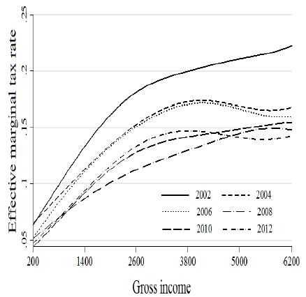
We start this discussion by showing the progression in the effective marginal tax-benefit rates. First, let us recall that, for a given level of gross income, the effective tax rate shows the expected total taxes (direct and indirect) for an additional earned peso.17 For instance in 2012, those with an equivalent gross income of 3 800 MXN, must pay a total tax of about 0.13 cents for an additional earned unit of income. Figure 7 shows that this effective tax rate has decreased drastically during the last years. This can be potentially explained by a combination of factors such as:
1) The increase in the size of the informal sector (enabling tax avoidance and regulations);
2) Corporate tax evasion and ineffective corporate tax alleviation (as confirmed by Kumler, Verhoogen, and Frias, 2013).
Source: Authors’ calculation using ENIGH data from the corresponding years.
Figure 7 Effective marginal tax rate
These results indicate an urgent need to revise the Mexican tax system to enhance its social and distributive efficiencies. In Figure 8 we show the effective marginal benefit rate. It can be seen in this figure that the marginal decrease in benefits resulting from an additional earned peso is higher in 2012 than in the other years, especially for the poor. This result requires some clarifications. First, the decrease can be greater if the group receives a high level of benefits. Of course, this was the case for Mexico in 2012. Second, with the presence of an efficient mechanism for targeting the poor, if they start earning a greater income they will lose assistance through a decrease in benefits (i.e. an increase in the tax-burden). These two combined effects make the decrease in effective marginal benefits steeper in 2012. This result shows the progressive nature of the distribution of benefits in Mexico, regardless of the real impact of benefits on the levels of poverty in the country. Scott (2014) researched the effect of Mexico’s fiscal system in reducing inequality and shows that this effect increased slightly between 2008 and 2010. It could be argued that “this reflects the low redistributive efficiency of indirect subsidies when compared to direct transfers” in the households and contributors (see Scott, 2014: 8, 12). Our findings are in line from Scott (2014) for most of the decade we examined, which strengthens our findings of an increasing progressivity fueled by cash-transfers and a low tax-burden in lower groups of income.
Source: Authors’ calculation using ENIGH data from the corresponding years.
Figure 8 Effective marginal benefit rate
Has the Mexican fiscal system become more progressive in recent years? To answer this question, we use the local and global measures of the progressivity approach explained in section 3.1, to test the local progressivity of the fiscal system. We show the liability and the residual progression curves in Figures 9 and 10.18

Source: Authors’ calculation using ENIGH data from the corresponding years.
Figure 9 Liability progression curves LP(x)

Source: Authors’ calculation using ENIGH data from the corresponding years.
Figure 10 Liability progression curves LP(x)
Starting from these results and applying expressions (5) and (6), an improvement in the local progressivity of the Mexican fiscal system can be seen, especially for the bottom part of the distribution, since we find that LP (x) < 0 ∀ x over the 202-2012 period. This can be seen in Figure 9 as a shift to the right of the liability progression curves over this period. For the residual progression, Figure 10 shows an overall negative movement for RP (x) < 1 ∀ x with a greater effect in 2012 for the lower incomes (i.e. a shift to the right of the 2012 curve up to a level of $3,000 pesos) and regardless of the level of taxes and benefits. This contrasts with the results found in Scott (2014), where in 2010, he found that indirect subsidies net of indirect taxes became more negative (regressive) after the first population decile in the Mexican distribution of income. A good reason for this contrast could be the lack of a common support of comparison in his analysis.
As indicated in the theoretical framework section, the absence of the common support of comparison of the distribution of gross income across years may bias our conclusion. Progressivity indices should not be compared whenever there is a change in the distribution of gross income between the two years being compared. Even the comparison of inequality indices could be biased, leading to misleading signs of deep and volatile short-term changes, such as the one found in the 2008-2010 analysis in Scott (2014).
To remedy this problem, we use 2012 as the pre-tax income base year (using gross income in our case) and then we estimate the expected post-fiscal income (net income) in 2012 using the fiscal system of 2004 or 2008. To estimate the counterfactual vector of net incomes of 2012, based on the fiscal system of a given precedent year, we use the locally linear non-parametric estimation approach as stated before, with the expected non-parametrical expression
This estimate gives us the tax/benefit an individual i would have faced if the tax/benefit system of 2004 and 2008 had been applied in 2012. Although, this procedure does not allow us to calculate the expected local variability of net income, local variability does not affect the estimation as much as the progressivity indices. Figure 11 shows the expected net impact for the tax-benefit systems in the years 2004, 2008 and 2012. As can be seen, while the tax-benefit system of 2012 was relatively more progressive, in that it benefited the bottom part of the income distribution to a greater extent, it was also less efficient at collecting more taxes at the top part of the distribution (see Figure 7). However, since the social welfare measurements are more sensitive to the bottom part of the distribution, the net impact is an increase in progressivity, in line with expression (16) which says that a fiscal system is progressive if and only if IG X -IC X-T+B > 0.

Source: Authors’ calculation using ENIGH data from the corresponding years.
Figure 11 Expected net impact based on tax-benefit system for different years
Now, we present and discuss the global progressivity indices with and without a formal common support of comparison, and our results seem to confirm that the fiscal system is progressive in each of the years studied. Although the increase in the progressivity of the fiscal system is apparently small during these years, one must be careful in coming to this conclusion. As indicated in the theoretical framework section, the absence of the common support of comparison of the distribution of gross income across years may bias our conclusion. Without this support, progressivity indices are not directly comparable if the distribution of gross income changes from one year to another. Results concerning the evolution of the fiscal system’s progressivity, without using the formal common comparison support are reported in Table 3 and Figures 12 and 13. This evidence is confirmed by the second theorem stated in expression (7) and empirically proved using expression (13). It can be seen that the progressivity curves comply with the positive condition TR(p) > 0 ∀ p.
Table 3 Evolution of fiscal system progressivity in Mexico.
| Year | TR approach | IR approach |
| 2002 | 0.0485 | 0.0586 |
| 2004 | 0.0512 | 0.0593 |
| 2006 | 0.0453 | 0.0524 |
| 2008 | 0.0469 | 0.0507 |
| 2010 | 0.0561 | 0.0606 |
| 2012 | 0.0564 | 0.0606 |
Source: Authors’ calculation using ENIGH data from the corresponding years.


Source: Authors’ calculation using ENIGH data from the corresponding years.
Figure 13 IR progressivity curves
It may be helpful to explain here why we observe that the TR(p) curve becomes negative at the top range of percentiles when using 2012 as the reference year for pre-tax income as formal comparison support (Figure 12 and 13). Our investigation shows that this is caused by the large benefits received by a few rich households, mainly in the 2004 survey. However, this makes the concentration curve of benefits lower and constant for a larger part of the distribution. As a result of these outliers, the difference between the concentration and Lorenz curves becomes negative.19
In the Figure 12, you can also observe a large increase in the progressivity of the fiscal system in 2004, compared to 2008 and 2012. A second finding concerns the reversal in the rank of progressivity. Figures 12 and 13 depict how 2004 seems to be the year with the highest level of progressivity; meanwhile, by considering the common support of comparison for the year of 2012, and dropping the extreme outliers in the survey, this effect is off-set (see Figures 14 and 15). Finally, it is important to note that in Figures 12 and 13, the impact of changes in pre-tax incomes on progressivity indices is no longer ignored.20


Source: Authors’ calculation using ENIGH data from the corresponding years.
Figure 15 IR progressivity curves Base pre-tax income year: 2012
Our results are directly comparable to those obtained for Canada in Araar (2008) -see Table 5- where the common support of comparison is used (with 2005 as the reference year for pre-tax income). Canadian findings show declining progressivity level in the tax-system between 1996 and 2005 with indices of 0.147 and 0.122 respectively. Using the TR approach, the level of progressivity increased slightly, with indices of 0.1152 in 1996 and 0.1222 in 2005. These results confirm the importance of taking into account the issue of pre-tax incomes when making formal comparisons to determine fiscal policy design.
Table 4 Evolution of the fiscal system progressivity in Mexico. Base pre-tax income year: 2012
| Year | TR approach | IR approach |
| 2004 | 0.0373 | 0.0422 |
| 2008 | 0.0529 | 0.0583 |
| 2012 | 0.0564 | 0.0606 |
Source: Authors’ calculation using ENIGH data.
Table 5 Evolution of the fiscal system progressivity in Canada. Base pre-tax income year: 2005
| Year | TR approach | IR approach | TR base | IR base |
| 1996 | 0.1470 | 0.1580 | 0.1152 | 0.1300 |
| 2000 | 0.1231 | 0.1350 | 0.1161 | 0.1296 |
| 2005 | 0.1220 | 0.1306 | 0.1222 | 0.1299 |
Source: Araar (2008).
Tables 4 and 5 show that indices for progressivity are higher in Canada than those obtained for Mexico, using both TR and IR approaches and using a formal common support of comparison. For Canada, the level of progressivity was found to have increased over the period studied. However, in Mexico the level of progressivity was lower than in Canada, as was the degree of growth in progressivity.
It is obvious that Canada’s fiscal system has a greater impact on its redistributive fiscal system than Mexico: from the pre-tax situation to the ex-post fiscal condition, the decrease accounts for 27.9 points of the Gini index in the case of Canada, while in Mexico, our study shows a reduction of just under 6.4 points (as shown in Table 1).
For the United States, Piketty and Saez (2006) provide estimates for a longer period of analysis, examining federal tax rates by income groups from the 1960s until 2006, with special emphasis on the top income groups. They use a type of incidence estimation for taxation rates according to income fractiles (i.e P0-90, P90-95, ..., P99.95-100)21 and report top income shares both pre-tax and post-tax incomes, but they do not adjust for the lack of common support of comparison. In another contrast with our study, they include other taxes such as corporate, estate, gift, and payroll taxes, but despite these differences, their findings are in line with our research, although ours shows a lower degree of progressivity of the fiscal system when a formal common support of comparison is used and outliers are dropped. The degree of progressivity of the US federal tax system has declined dramatically since then (Piketty and Saez, 2006).22
In the case of some developed and middle-income countries (including Mexico), research from OECD (2012) presents relevant information concerning the tax-burden incidence and progressivity for groups of contributors. According to this research, Mexico obtains a higher share of total taxes from wage earners than do other OECD member countries. However, this research shows that across the OECD countries, on average, three quarters of the reduction in inequality is due to transfers and the rest to direct household taxation. Thus, it seems that transfers seem have a greater effect on inequality than do taxes. In some countries, cash transfers are small but highly targeted to those in need such as the Mexican case. After comparing the results of this paper with our results, it can be argued that the low capacity of redistribution via benefits (i.e. means tested cash benefits, mainly) in Mexico is due to the scarce coverage of social programs, due to Mexico’s incapacity to tax the top household level of incomes.
5. Conclusion
This paper focuses on how the progressivity of Mexico’s fiscal system has evolved, as well as changes in inequality and in the polarization of preand post-fiscal incomes between 2002 and 2012. In addition to the macroeconomic performance criteria, the change experienced in the distribution of wealth over this time period must also be assessed and analyzed. It has been argued that macroeconomic performance may help to increase the overall wellbeing of a population, but it does not guarantee a more equitable distribution of wealth. Over time, many factors can contribute to the reshaping of the distribution of income. In addition to economic growth, other issues such as market forces, population endowments and fiscal system measures can have an important influence on the distribution of wealth. In Mexico, both the fiscal system and social programs should be used as crucial tools for reducing income disparities more quickly.
In general, the fiscal system had a positive impact on the income of the bottom part of contributors in the distribution. However, even though the tax-benefit system in 2012 seems to have benefitted the bottom part to a greater extent than in the other years studied, it was also less efficient when collecting taxes to the top part of the distribution. The social welfare measurements implemented were more beneficial than the fiscal system to the bottom part of the distribution. Nevertheless, the impact on the reduction of inequality found is null, despite the increase on progressivity in taxes.
The conclusions and remarks drawn from this study can help policy-makers choose and apply fiscal policies that will have a greater impact on progressivity. The other contribution is the development of methods to assess the progressivity of the fiscal system. Our method of distributive analysis, which we applied to Mexico’s fiscal system and social benefits program in this study, can be replicated for other countries or at the regional level. Finally, we would like this research to inspire investigations on the impacts of a wide variety of taxes and benefits through time on specific groups of contributors, such as entrepreneurs, self-employed individuals or the poor, in order to improve both the fiscal and social policy agendas of governmental action.