


 text new page (beta)
 English (pdf)
 Article in xml format
 Article references
 Send this article by e-mail
 Cited by SciELO
  Similars in
SciELO
Similars in
SciELO 
 Permalink
Introduction
In the current economic situation, where the interest-rates world-wide are at historical lows, and due to a 2008 mortgage crisis, many investors switched from debt derivatives into a government obligations, where the security provides a stable fixed income return, compared to an equity market where the fluctuations of the stock prices can be hardly predicted and the dividends payout are not stable. In many cases investors require stable returns and looking at investment at the government obligations, but there are many factors that have to be looked at and there is a need of a bond yield factor analysis so that investors know at which factors to look during the analysis of the opportunities (Diebold, Piazzesi and Rudebusch, 2005). There are a plenty of studies available that answers the questions on the presence of the factors that influence the corporate bond yields (Israel, Palhares, & Richardson, 2017; Bai, Bali and Wen, 2019), These study shows the factors that have a significant influence on the government obligations yields. Financial institutions have sufficient resources to hire the analyst that can perform investment analysis on the government obligations, where the private investors are not possessing with such funds. This study provides the factors and magnitudes with which the bond characteristics contribute to the yield to maturity, which can be used in the investment analysis by private investors and institutional at the same time.
In many papers the key topic of the research is focused on corporate bonds, but not to much on government ones. Especially, when the obligations contribute to a large proportion of investors' portfolios (Bai, Bali and Wen, 2016; Vukovic et al., 2020a; Moinak et al., 2020b). What makes a research based on government obligations to be an interesting topic, especially in the current market conditions? In Canada the volume of quarterly bond outstanding has been growing over the period from 2009 until 2015, where the average volumes outstanding grew approximately on 50% over this period, accounted to the 70 billion of Canadian dollars in government debt placed on the market in 2015 (Fontaine, Garriott, and Gray, 2016). Where the convertible bonds are also popular and the amount outstanding increased almost three times over the period of 2012-2015, accounting to 157 billion Euros. The current market situation makes the topic of government obligations to be a very important, as many funds are poured into this asset, as bank deposits are at its lows and the stock returns are under a great uncertainty due to an unpredictable behavior.
Due to a crisis many investors suffered from illiquidity during the pick of it, so that liquidity risk started to be one of the key aspects in investment analysis and also can provide a significant level of returns (Huang, Huang and Oxman, 2015). In many cases the government obligations are bought not only by institutional investors and financial institutions, but also purchased by the central banks world-wide. In 2012 the European Central Bank possessed 17% (42.7 bln. Euros) of the total amount outstanding of the Greek government obligations available (Trebesch and Zettelmeyer, 2018). Many researchers focus on the liquidity factor exclusively, where this paper takes into account the existing work on the liquidity premiums and adds an understanding of other factors that are significant in determination of the bond returns, providing the breakdown of yield to maturity composition.
There are a plenty of bond characteristics such as: coupon payments, coupon frequencies, amount outstanding, credit ratings, liquidity, maturity and the issuer country. The term structure of interest rates provides a theory of the about the maturity premiums, which explains that investors obtain an extra return for possessing the risk during a longer period of time (Bodie et al., 2013).
Many of the existing studies analyze the effect of the changes in the agency ratings and the possible concerns in the financial markets about the reliability and the significance of the credit ratings (Cooke, & Bailey, 2015; Baum, Schafer and Stephan, 2016) what became an important topic which is highly discussed, due to a major failure in 2008 during the mortgage crisis. However, the actual magnitude of the affect that the credit rating premium brings to investors is not analyzed. The market players are left only with the theoretical approach without possessing the average market behavior which can greatly simplify the investment analysis. Also, as there has been a major financial recession worldwide, the current state of the financial market is under the great concern and the study explains the current behavior of the bond returns providing an inside in the relation of the credit ratings and bond yields.
This paper provides an OLS regression (based on the cross sectional data at the current period of time) of bonds yield to maturity and the macroeconomic factors, which provide the coefficients that explain the effect of each significant indicator on the yield to maturity of the government obligation in United States (US) and European Union (EU). This could be used to explain the interrelation between the characteristics and the returns and show which premiums are higher, what makes it important to pay attention to them making the investments. Also, as there always a risk-return trade-off, the coeffect in the model represent the higher risk associated with the premium impaled in the yields; as well as, checking the difference in the debt markets between the US and EU markets. As the popularity of the government obligations investment is growing, both in the private and institutional divisions, as the bank deposits are losing its attractiveness due to a lower return. The factor analysis of the bond yields is useful for investors by providing the simple method of investment analysis to obtain a desired level of return. Also, financial markets worldwide have changed significantly due to a couple of the financial crises and increasing political tensions, makes it important to check the current composition of the bond yields and the method which is used hear can be applied when the current results are outdates. Regression model which is used in this study has a good fit with the data, what shows that the method can be implied to other economies and can implied during the investment opportunity analysis and portfolio composition to check the premiums implied in the bond returns.
Literature review
In the past years the financial situation in the world has changed dramatically and the investors a constantly seeking for the low-risk stable investments. Due to the changes in the economic situation there is a need to examine the key factors that affect the returns on such investments. As many studies propose, in the period of declining interest rates, even negative in some cases, the investors are constantly looking for opportunities to perform a yield pick-up on the foreign markets, despite the fact that the higher yields provides often more risk; or investors choose to go for longer duration investments that reward its holders for a longer period of exposed risk (Ammer et al., 2018). Recently, there has been a work done with the help of time-series analysis that contributed to the research of the liquidity risk on the high-yield bonds affect before and after the crisis period, where the results showed that liquidity risk is crucial especially in the bond pricings (Zeng, 2018). In many cases, the investors that choose to pursue with the government obligations in portfolio, tend to hold to a maturity, as there is almost twice the number of buy orders on the debt market compared to a sell orders (Schultz, 2001). There has been a research in the sphere of searching the factors that responsible for the bond returns (Driessen, Nijman,. and Melenberg 2000) have proposed a multi-country model that takes into a currency hedged returns, where the key factors that were included is the risk measures. The topic of the rating agencies announcements and issuer grading especially the way it affects the prices on both the stock market and debt market. Hite and Warga (1997), carried out a research on the correlation between the changes in the agency gradings and the bond prices, where the key results showed that the there is a response of the prices especially when the grades drop down to a non-investment grade. In many cases, researches have tried to provide an alternative measure of stock or bond liquidity, at the same time checking the relationship between the liquidity measures and returns or prices of assets. One of the proposed measures is a "latent liquidity" which provides a possibility of forecasting a trading cost, volume and other paraments associated with the asset. To be able to construct such index, authors used not only a classic measures of trading prices, but also included parameters such as: volume, amount outstanding, age, ratings and interest coupon payments. (Mahanti et al., 2008)
As recent research shows, investments in government obligations can bring a higher return than ordinary bank deposit. However, still investments in government obligations will be stable and secure, especially when choosing the countries with a high agency rating (Vukovic and Prosin, 2018). In another study, done by Choi and Kronlund (2018), at the current low-risk environment many funds are in the consideration of choosing the higher yield investments in the era of low interest on the markets compared to their general standards of investment risk, and could suffer from a lower liquidity and greater associated risk with the investment. Due to these facts, there is a need to analyze the factors that affect the bond returns, especially yield to maturity and which factors affect the returns the most; so that investors can pay a great attention when they analyze the investment opportunity in the government obligations. In many insurance companies, asset managers are focusing on returns higher than a standard benchmark making them hunting for yields and composing their portfolio with higher rate obligations compared to the stable high rating investments, the common risk measure is an agency rating of the obligation which are used to compare the safety of different issuers, and they are not affected by liquidity and market conditions what explains the stability and the returns on the government bond (Becker and Ivashina, 2015). In the research done by Burger and Warnock's (2018), the analysis of investors preference in the choosing of government debt securities is done, where it has been compared the percentages of the different currency securities in portfolios and the results showed that the investors focus not only on the local bonds, but also prefer to include the foreign investments in to portfolios. These investor preferences can be supported by adding extra factors that will support the better investment analysis, which will contribute to a higher return. There is a good proxy for analysis of the general activity on the debt market where the amount outstanding of the government obligations (Aggarwal, Bai and Laeven,2018).
To be able to pursue a high-quality investment analysis, investor has to obtain high-quality information about the future investment. In the case of the of the government debt securities, one of the crucial information parameters is default risk. The common risk characteristic of the issuers is the agency rating which provides a grade of the stability of the company or an organization (Faerber, 2001). The agency rating grades affect both stock and bond returns, where the low-bond rating provides an insight into instability of the issuer and shows that the issuer with a high probability of default; and if there was a change in the rating grade the market will react by the changes in prices and yields of the changed issuer. During the 2008 world financial crisis, many institutions and private investors suffered from unreliable information that caused the world crisis to begin, which had a great effect on all economies worldwide (Sinclair and Timothy, 2010). Despite, the nature of the rating grades during 2008, the stock and bond returns are still having a significant correlation between the grades (Sehgal and Mathur, 2013).
Robin Greenwood and Dimitri Vayanos (2014) proposed that with increased supply of the long-term obligations, the price of the security falls die to a decrease in overall demand, what can make a plausible factor in the determination of the factors affecting the bond returns. The bond convexity is another crucial factor that relates the bond prices and interest rates. It is a crucial, as its duration makes the bond with a greater sensitivity of the debt instrument prices to a change in interest rates (Malkhozov et al., 2016). In another study, the relationship between the bid-ask spread and the earning announcements on the equity market were done by the Acker, Stalker and Tonks (2001). The following relation was found that on the day of earnings announcements the bid-ask spread is falling and volumes and return rises as follow. As the bid-ask spread can largely affect the returns on the stock market, this relation has to be checked on the debt market to study how the bid-ask spread can contribute to the returns and to what extent.
The existing research suggests that the returns on obligations do not follow a simple monotonic function, but rather have a pick at certain maturities (Fama, 1984). This proposes that the yield to maturity doesn't grow at the steady rate. However, it has picks at certain maturities what shows a necessity to evaluate factors that affect the yield to maturity. This will propose a clear investment analysis factors to maximize the investors returns. Also, in the work done by Hopewell and Kaufman (1973), the general rule is that for the longer maturities .the changes in the obligation prices are larger if there is a change in yields; however, there are some anomalies where the longer term maturities affected less than the shorter maturities. Despite the anomalies mentioned by the previous study, in the article by Litterman and Schenkman (1991) three factors were proposed that explain the returns on the government bonds, this factor are as follow: level, steepness and curvature; where these factors are particularly useful for the choosing the hedging strategies especially in the different market segments and instruments. The yield curve has a major dependence on the coupon payment, if the coupon payments is changed by the duration of the obligation, what affects the yield to maturity (Cumming, Fleming and Liu, 2015). Also, yield to maturity assumes that all coupon payments are paid at the set constant time and evaluates the present value of all cash flows till the maturity (Asonuma, Niepelt and Rancière, 2019).
The liquidity is a key concept in evaluation of investments in affecting the returns, as also has a crucial aspect when the investor tries to sell the asset. However, there is a crucial difference between the liquidity and liquidity risk. The liquidity determines the possibility of a holder to sell a big volume of assets on the market with low transaction costs and in short period of time, where the liquidity risk refers to the relationship between the liquidity of the asset and its expected return (Ng, 2011). According to Lin, Wang and Wu (2011), the liquidity risk is not situation where investors will not be able to sell the obligation on the market, but rather due to a low demand, they will suffer from a loss in prices due to a lower demand, which follows by the lower prices on the market. The theory shows that, the investor should be rewarded by a greater overall for choosing the asset with lower liquidity compared to the more liquid assets. The liquidity premium is a key determinant in the prices and returns not only on fixed-income markets, but also on the money market. Pástor and Stambaught (2003) have analyzed the relationship between the liquidity risk and the expected stock returns and proposed, that if the asset is under a strong influence of liquidity risk, it provides a higher returns for its investors; as well as, proposed to check if such a behavior holds for other markets including the debt market. Despite the fact the equity market tends to be more liquid than the debt market, the liquidity factor in returns still plays a crucial role that needs to be taken into account (Lin, Wang and Wu, 2013). Joslin and Konchitchki (2018) proposed a research that analyzed four factors that influence the term structure which included the price of risk on the market, macroeconomic situation, volatility and convexity.
The study of the bond agency ratings was discussed for a vast period of time, many studies searched the effects of the bond ratings (Vukovic, Lapshina, & Maiti, 2019) changes announcements on the stock and bond returns. In 1977, Hite and Warga have discussed the results of the downgrade of the ratings and its response to the market characteristics. Chen, Lesmond and Wei (2007) carried out the research that cheeked couple of the liquidity measures which supported that the liquidity is key factor on the yield-spreads, which are suitable not only for a high-grade security but also for speculative level ones. The agency ratings play an important role in the bond returns, with increasing grade level investors are faced with less credit risk what lowers the premium on the investment (Spiegel, and Starks, 2016). Amihud and Mendelson (1986), argued that liquidity is highly correlated with equity return, where the measure of liquidity was proposed the bid-ask spread. The higher bid-ask spread shows that the asset suffers from the liquidity problems and there should be a liquidity premium on this asset (Wulandari, Schhfer, Andreas, and Sun, 2018). In some cases, if there has been a downgrade of the country credit rating, players on the market can start speculating on the fundamental information regarding the country currency, what will force largely affect the bond returns as well (Baum, Schafer and Stephan, 2014).
Despite the bond characteristics as major effect on their yields, there is also a significant influence from the macroeconomic environment on the bond market. Many researchers try to decompose the risk premiums in to specific categories. The topic of government obligations and macro factors has been in particular interest in the financial sphere, especially due to a couple of the severe financial crisis (Aguiar and Gopinath, 2004). In many studies, researchers test the methods of (Vukovic et al., 2020b, Maiti et al, 2020a) the interest rates and the yield curve forecasting, what makes the interest rates to be one of the key factors in the bond returns (Diebold and Li, 2006). Interest rates have a major effect on the bond yields, which capture an extra return for the interest rate risk and that can be a good factor in forecasting the bond returns (Ferson and Harvey, 1991). Central banks have regulatory instrument interest rates, where the economies money supply can be controlled. By changing the interest rates, countries adjust the cost of borrowings for firms and investors what reduces the spending in the economy, while increasing the attractiveness of savings (particularly the deposits and investments in bonds). This shifts the demand for investment instruments (Engel, 2016). In many cases the interest rates is a good benchmark for the expected bond returns. With increasing interest rates, yield to maturity of the government obligations grows by dropping the prices due to a decreased demand for the government obligations and the bank deposits become more attractive due to a higher interest rates paid on them (Cox, Ingersoll and Ross, 2005; Lustig, Stathopoulos & Verdelhan, 2016). However, some countries implied negative interest rates in the economy. This measure was implied to control the inflation in the economy and to increase the holdings of the government obligations by the Central banks to keep the money supply constant in the economy (Bech and Malkhozov, 2016).
The country growth rate also has a significant influence on the bond returns (Ang and Piazzesi, 2000). Economic growth has a direct relation to the bond yields, with increasing economic prospective in the economy, the stock investments are increasing its attractiveness due to an increased return. Bond yields are also increasing, as the investors are switching from the low-risk stable investments to a equity investments. Such situation forces the bond yields to go up as well as demand is falling down and forces the prices to lower as well (Nakamura, Sergeyev and Steinsson, 2017). In some other studies, researchers proposed and successfully checked that the behavior of the bond yield premiums has a significant predictive power of the future economic growth and shows that there is a significant relation between the economic growth and bond returns (Bleaney, Mizen and Veleanu, 2016).
Debt to GDP ratio is another commonly known macroeconomic factor that has a major effect on the bond yields with a positive correlation (Lemmen, 1999). With increasing debt burden by the government, the investors that possess the state debt securities are subject to a higher default risk as the government has a higher default and credit risk for which the investors have to be rewarded (Blanchard, Mauro and Acalin, 2019). As the current study suggests, with increasing debt to GDP in the country, the government obligation returns increase in both long and short run perspectives (Poghosyan, 2014). From other side, there are studies where the opposite economic theory is proposed, as the debt to GDP increases the uncertainty in the economy increases as well, what shifts the demand to the stable debt instruments increasing its prices what forces the returns on the government to go down (Bernoth, von Hagen and Schuknecht, 2012).
Methodology
Data description and sample statistics
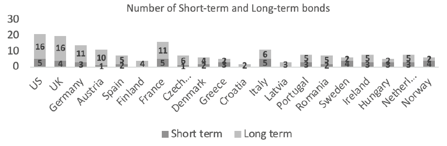
The dataset consists of 175 observation, from US and EU debt markets with a wide-range of maturities with current prices as on 3rd April, 2019. The criteria for selection countries in EU (out of US data) in dataset where EU countries with the highest number of issued treasuries. Maturities range from 1 month up to 600 months (50 years), where there 37 short-term government obligation (less than or equals to a year until maturity) and 138 maturities with time to expiration over one-year period. Figure 1 shows that in most of the countries have the long-term debt outstanding, with some countries possessing only the long-term debt on the market (Finland, Croatia, Latvia); where Sweden, Hungary, Norway and Greece possess more short-term government obligation than the long-term ones. This data shows that most of the countries are focused on the long-term issues of government obligations and try to spread its debt burden over the years, by varying the maturity. For example, US and UK (for the UK, data were collected in period before Brexit) have a 16 long-term bond traded on the market, Germany and France have 11 of them, where the short term bonds currently traded on the market are much lower in quantities: US and France have 5 b bonds each, UK had 4 bonds and Germany has 3 bonds.
Source: Thomson Reuters (2019).
Figure 1 Number of short-term and long-term bonds chosen for the analysis in each country.
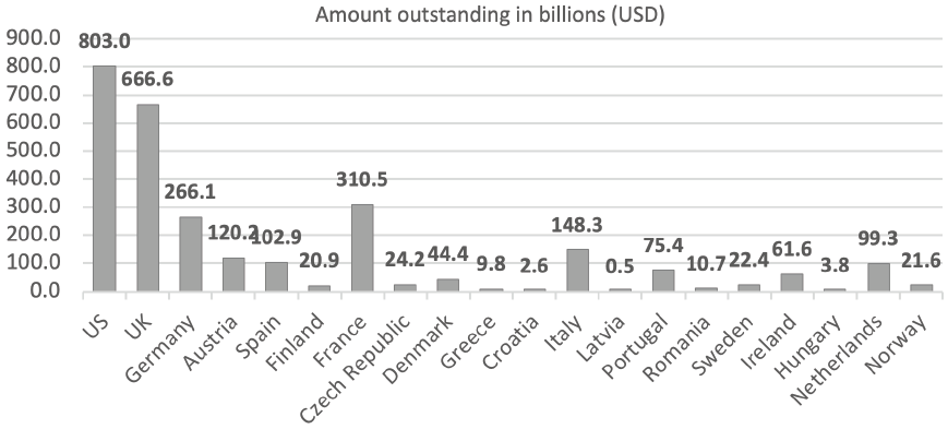
Combining the obtained data from Figure 1 and Figure 2, countries with the highest debt outstanding, possess the highest number of long-term bonds available on the market. The US and UK take up in the lead across the highest owners of debt, with 803 bln. USD and 666 bln. USD respectively; and with the highest number of long-term bonds outstanding which account to 16 long-term bonds for both countries. When looking at the countries that have only the long-term bonds trading on the market, the total amount outstanding of the debt in these countries is one of the lowest analyzed in this research. Latvia has only 0.5 billion dollars outstanding and the highest out of the countries which have only the long term debt is Finland with 4 long term bonds trading, which account to 20.9 billion dollars outstanding. Countries like Sweden, Norway, Greece and Hungary focus more on issuance of the short-term obligations that are traded on the market at the current period of time.
Source: Thomson Reuters (2019).
Figure 2 Amount outstanding in USD of government obligations across the analyzed countries.
Due to a fact that bonds that are trading on the market at the current period of time are issued on different dates and years, that bonds from the sample have a different economic conditions on the date of issue, what affects their interest rate payments. Due to this nature, in many cases bonds with shorter maturities can provide a higher coupon payment than a bond with a longer maturity in the same country (as a paradox by interest rate theory). In US market, the 30 years bond can provide 3% coupon payments where the 14 years government obligation can provide in coupon 6.25% (see more about similar paradox cases in Bodie et al., 2013). The same situation can be seen in UK where the 12-year bond can provide 4.75% coupon payment, and a 30-year bond only 1.5%. Due to financial crisis during which countries raised the interest rates, during this period, bonds with a higher yield where issued. Soon after the crisis, economies came back to a more stable growth rate, the interest rate lowered and the coupon payments declined back to a before crisis period.
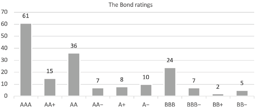
In the chosen sample, the greatest number of bonds account to the AAA rating, as the US and EU markets are one of the most developed and include one of the most stable countries world-wide. The rating for this research were divided into three sub-categories. The data collected from the market (Figures 3 and 4), shows that the categories are not evenly distributed and most of the obligations analyzed fell into the highest rating criteria and shows that on the analyzed markets, issuers are graded as the upper investment grades, where the most of the issuers and its outstanding debt is subject to a low default risk, providing the investment to be stable and moderately risk-free.
Source: Fitchratings (2019).
Figure 3 The bonds rating chosen for the analysis and its frequency in the sample.

Models
In many papers that exist in the sphere of finance research, the key concern, is the way liquidity affects returns or prices of assets. The assets that are mainly analyzed are corporate debt instruments or the stock market, while this research is focused on the government obligations, which can be affected by the common measures in a slightly different manner.
The population that this research can be extended to is all government obligations in United States and European union that are traded at the current period of time on the debt market. The research is based on the convenience sample, as there care certain difficulties in the data collection. As the market data was collected from the Thomson Reuters terminal, in the export files for a certain number of countries the data is missing, forcing this observation to be excluded from the sample. Where the research sample contains 175 observations, with US market and 19 European Union countries. Each observation consists of a government obligation, with different characteristics which include the following factors that are considered in the regression model.
The data available on Thomson Reuters is related to the current trading prices on the market from different brokers, with different dates of issues, what makes the interest rate payments on those bonds to be inconsistent, as they all were issued at different economic environments. To stabilize the returns the market adjusts the prices on the assets to keep the overall return consistent with the general market tendency. The key aim of this research is to find the key factors that can describe the yield to maturity (YTM) of the government obligations in EU and US, where the dependent variable will be YTM. YTM is taken as it is one of the common measures that is used to describe the total bond return if the asset will be held to the end of maturity (Bodie et al., 2013). Where the YTM is calculated by the following formula:
Where the following notation is used:
YTM: yield to maturity
C: coupon
FV: Face value of bond
P: price of bond
T: time to maturity in years
In many cases the coupon payment is handed out to the holders more than once a year, in this case YTM has to annualize to the frequency of coupon payments a year. Using the following formula:
Where the following notation is used:
Adj. YTM: annualized YTM to the frequency of coupon payments per year
n: frequency of coupon payments per year
One of the key factors that is considered in this research, is the liquidity factor which has a variety of the possible indexes used. In one of the recent papers, done by Vadim Konstantinovsky and Bruce Phelps, the directors of the Quantitative Portfolio Strategy Group of Barclays in New Your, proposed a measure of "Liquidity cost score (LCS)" that is used by the traders, and represents liquidity measure as a trading cost. The following formula is proposed for the Liquidity cost score calculation:
(Konstantinovsky and Phelps, 2016)
Were all the prices are taken from the market data from brokers.
Occasionally, the prices on the market for the short-term treasury securities (in this research, the short-term US government obligations) are quoted in terms of its discount rates, so to obtain a price the discount should be converted to a dollar value. For the conversion the following formula is used:
Where the following notation is used:
Price: the bid/ask price calculated from the market discount rates
FV: face value of a bond
maturity: the proportion of the year that is left until maturity (days/360)
To be able to find the factors that affect the bond yield, the regression analysis is used. The method is going to be an Ordinary least squares regression with a multi-factor characteristic of bonds available on the market at the current period of time, to capture the current situation of the market behavior. The regression equation fits the following form:
Where the following notation is used:
α:the y-intercept
β1,j:the regression coefficent of the factor
Government obligation charecteristic: independent variables
ε: error term
(Koijen, Lustig and Van Nieuwerburgh, 2017)
The key concept of this research is to provide the key factors that influence the bond returns on the market at the current state of the world-wide economic situation. The Government obligation characteristics for the regression are chosen to be the following:
Table 1 List of Independent variables that determine the adjusted yield to maturity of the bond
| Characteristic | Description | Independent variable (Notation used in the regression equation) |
|---|---|---|
| Coupon rate | Interest rate paid on the bond in decimals | Coupon |
| Agency rating | Dummy variable for the
agency rating grade, the rating are pulled into groups with the following characteristic. Upper investment level (AAA, AA+, AA, AA-), medium investment grade (A+, A,A-) and all the other grades are left to a lower and speculative grade pool. (Fitchratings.com, 2019) |
Uinv Minv |
| Amount outstanding | Total value of the bonds
released on the market; the value is turned into billions. |
Amoinbil |
| Liquidity index | Liquidity cost score | Liquidaskbidbid |
| Maturity | Maturity in years | Maturityinyears |
| Issuer country | In to the regression the
US dummy is added, to analyze if there is a significant difference in the returns between the EU and US markets. |
USdami |
| Coupon frequency | Frequency of the coupon payments per year | Couponfrequencyperyear |
Source: arranged by authors
The factors in the table 1 above are used to determine the factors that determine the adjusted yield to maturity of the bond and used as a bond characteristic for the regression model. The second regression model is done on the basis of the macroeconomic factors, to determine the key independent variables that affect the yield to maturity, with the following regression equitation:
Where the following notation is used:
α:the y-intercept
β1,j: the regression coefficent of the factor
Macroeconimic charecteristic: independent variables
ε: error term
(Koijen, Lustig and Van Nieuwerburgh, 2017)
The second model represents the macroeconomic factors affecting the bond yield returns, with the following factors that are used in the regression model:
Table 2 List of Independent variables that determine the effects of on the yield to maturity of the government obligations
| Characteristic | Description | Independent variable |
|---|---|---|
| Inflation | Inflation in the country of the issuer | Inflation |
| Interest rates | Interest rates in the country of the issuer | Interest rates |
| Country growth rates | Country growth rates in the country of the issuer | Country growth rates |
| Debt to GDP ratio | Debt to GDP ratio in the country of the issuer | Debt GDP |
The factors that are mentioned in the table 2 above are used as the macroeconomic characteristic in the regression model that determines the effects of on the yield to maturity of the government obligations in the countries chosen for the analysis. To be able to accept the model there following test should be carried out. Test for the heteroscedasticity: Breusch-Pegan test is used for the heteroscedasticity test, where the null hypothesis is that the variance is constant, where the absence of the heteroskedasticity is one of the key assumptions underlying the OLS for the coefficients of regression to be unbiased (Breusch and Pagan, 1979). Test for the multicollinearity: Absence multicollinearity is another assumption that has to be present for the OLS. The independent variables should be free from perfect correlation. The test for the multicollinearity is variance inflation factor, which is a common measure of the magnitude that the variance of the regression coefficients obtained from the regression is increased due to multicollinearity. The VIF factor should be less than 10, to be able to prove that the model obtained is free from the multicollinearity (Chatterjee and Hadi, 2012; Belsley, Kuh, & Welsch, 1980)
Results and Discussion
For the first regression all of the factors have been chosen that should influence the YTM. Despite the fact that the R2, is 0.7804, what represents a good quality description of the dependent variable by it regressors. However, amount outstanding in billions is not significant in the model providing the p(value) of 0.538. The amount outstanding is not significant in describing the Yield to maturity, due to a low relationship with the interest payments and transaction costs for both buyers and sellers.
As the amount outstanding is not significant in Table 3, this variable is removed from the model. The second variable which is not significant in the model is the coupon payments. This is due to multicollinearity between the independent variables. In Table 3, the coupon frequency and the coupon itself have a strong correlation, with the value of 0.5657. All of the other factors have a correlation less than the absolute value of 0.5, what shows that other factors are applicable for the regression.
Table 3 Regression results with the following factors: Liquidity, Bond ratings pools. Amount outstanding, Coupon payment, time to maturity in years, comparison dummy between the EU and US
| YTMadjysted | Coef. | Std. Err. | t | P>t | [95% Conf. | Interval] |
|---|---|---|---|---|---|---|
| Liquidaskbidbid | 1.066858 | .3295158 | 3.24 | 0.001 | .4162763 | 1.717441 |
| Uinv | -.0083878 | .0018524 | -4.53 | 0.000 | -.0120452 | -.0047304 |
| Minv | -.0105864 | .0026612 | -3.98 | 0.000 | -.0158405 | -.0053323 |
| Amoinbil | -8.84e-6 | .0000143 | -0.62 | 0.538 | -.0000371 | .0000194 |
| Coupon | .0005973 | .0004856 | 1.23 | 0.220 | -.0003614 | .0015559 |
| Maturityinyears | .0003028 | .0000899 | 3.37 | 0.001 | .0001253 | .0004803 |
| USdami | .0359305 | .002349 | 15.30 | 0.000 | .0312928 | .0405682 |
| Couponfrequencyperyear | .0087554 | .0012082 | 7.25 | 0.000 | .0063699 | .0111409 |
| _cons | .0021722 | .0017883 | 1.21 | 0.226 | -.0013586 | .0057029 |
According to the Table 4, and high correlation between the two factors one of the factors should be dropped from the regression model. As one of the key cash-flows associated with the investment in bonds is coupon payments, what should be taken into account in the model.
Table 4 Correlation matrix between the independent variables
| Correlation | Liquid~d | Uinv | Minv | Amoinbil | Coupon | Matur~rs | USdami | Coupon~r |
|---|---|---|---|---|---|---|---|---|
| Liquidaskb~d | 1.0000 | |||||||
| Uinv | 0.2219 | 1.0000 | ||||||
| Minv | 0.0169 | 0.4936 | 1.0000 | |||||
| Amoinbil | 0.4171 | 0.0086 | 0.1205 | 1.0000 | ||||
| Coupon | 0.2419 | 0.0257 | 0.0944 | 0.1005 | 1.0000 | |||
| Maturityi~rs | 0.1567 | 0.2373 | 0.0374 | 0.0187 | 0.3518 | 1.0000 | ||
| USdami | 0.1936 | 0.2533 | 0.1250 | 0.0751 | 0.2101 | 0.1013 | 1.0000 | |
| Couponfreq~r | 0.0962 | 0.1127 | 0.0762 | 0.0841 | 0.5657 | 0.4581 | 0.3106 | 1.0000 |
If the coupon frequency is eliminated from the model, the following results are obtained as shown in table 5.
Table 5 model with eliminated variable with high correlation
| YTMadjysted | Coef. | Std. Err. | t | P>t | [95% Conf. | Interval] |
|---|---|---|---|---|---|---|
| Coupon | .0022136 | .0004919 | 4.5 | 0.000 | .0012425 | .0031847 |
| Maturityinyears | .0005268 | .0000956 | 5.51 | 0.000 | .0003381 | .0007155 |
| Uinv | -.0092671 | .0021034 | -4.41 | 0.000 | -.0134197 | -.0051145 |
| Minv | -.0129305 | .0030072 | -4.30 | 0.000 | -.0188673 | -.0069938 |
| USdami | .0393692 | .0025882 | 15.21 | 0.000 | .0342596 | .0444789 |
| Liquidaskbidbid | .8826693 | .336635 | 2.62 | 0.010 | .2180895 | 1.547249 |
| _cons | .00608 | .0019374 | 3.14 | 0.002 | .0022553 | .0099047 |
To accept the model the test on the heteroskedasticity and multiclonality are carried out. Where the zero hypotheses implies the homogeneity of variance and the alternative hypothesis is that the model implies heteroscedasticity.
As Table 6 shows, that p value is high and much greater than 0.05, what shows that the standard deviations in the error terms are not changing are not related with the independent variables. The second very important test that has to be carried out is the test for the multi-collinearity of independent variables, in the good model there should be an absence of the perfect multicollinearity. If the multicollinearity is present, one of the independent variables can be expressed as the linear combination of the other independent variable (one explaining variable can be predicted by the means of the other one).
Table 6 Results of the Breush-Pagan / Cook-Weisberg test for heteroskedasticity Ho: Constant variance
| Variables: fitted values of YTMadjysted |
| chi2(1) = 0.69 |
| Prob > chi2 = 0.4047 |
Table 7 shows, the variance inflation factors of the independent variables in the model. The values of the VIF factor are moderately low. The multicollinearity is confirmed if the variance inflation factor exceeds 10 (Chatterjee and Hadi, 2012). As the values of the VIF for the model are in average, 1.33 with the highest value 1.61 and the lowest 1.18 what confirms that there is no multicollinearity in the regression constructed.
Table 7 Variance inflation factors of the independent variables
| Variable | VIF | 1/VIF |
|---|---|---|
| Uinv | 1.61 | 0.621497 |
| Minv | 1.39 | 0.717030 |
| Coupon | 1.30 | 0.770607 |
| Maturityi~rs | 1.26 | 0.791279 |
| Liquidaskb~d | 1.24 | 0.805241 |
| USdami | 1.18 | 0.845846 |
| Mean VIF | 1.33 |
As the model obtained is free from multicollinearity and homoscedastic the model can be taken as a fair approximation of YTM. Table 3 shows the coefficients of the independent variables. The p(value) of the factors in model are all significant at 5% significance level (less than 0.05), and the R2 of this regression model is high and accounts to the 0.7109. LCS: Has one of the strongest effects on the yield to maturity. If the LCS is increased by the 1 unit, the YTM increases approximately by the 0.88 units in YTM if the other factors are kept constant. This shows that of the bid-ask spread is increasing investors are rewarded for a less liquid investment what shows that there is a liquidity premium, and investors are rewarded for taken a larger liquidity risk. As on average the bid-ask spread in the sample 0.15% and the average adjusted YTM is 1.2%. The regression coefficient shows that if the LCS is increased by the 0.01% the YTM increases approximately by the 0.0088% if the other terms kept constant. The regression model supports the literature review, which shows that at the current state of the financial market liquidity plays a crucial role in the bond returns. The investors have a choice between the assets with different level of liquidity, and they have to choose higher returns with a greater liquidity risk or a lower return but have a higher chance of selling the asset on the market if they have a need to do so. The Liquidity Cost Score (Konstantinovsky and Phelps, 2016) is a good measure of liquidity for the bond prices and is applicable for the investment opportunity analysis on the debt market. This factor in the regression model supports the theory of the liquidity premiums and adds to the study done by Pastor and Stambaught (2001), which were interested in the further research of the liquidity influence in the debt market.
The bonds are pulled into three pools, and the default value in the regression is the Lower investment grade pools. According to the coefficients in the regression the Lower investment pools yields higher return than the Upper and Medium investment grades. The medium investment grades bonds have a Yield to maturity lower by approximately 1.3% (keeping all the other factors constant), what confirms that with the lower grading, investors face higher default risks for which they have to be rewarded with the higher returns. However, the upper investment grades have yields lower than the lower investment grades by 0.93%, but the difference between the upper and medium investment grades is opposite. The medium investment grade yield lower than the upper investment grade by 0.37%. The regression model supports the general behavior of the bond yields with respect to the different credit ratings, the lower investment grade yields higher than medium investment grade (Spiegel, & Starks, 2016), but results in the obtained model show that upper investment grade provide a higher return than a medium investment grade. One of the key reasons that could be associated with such behavior, is if some of the countries in the Upper Investment grades should have been lowered in the agency ratings that is why the return for them is higher, but there is often a delay in the updates of the ratings grades what could cause the upper investment grade to yield higher than the medium grade if the other factors are constant (Broto and Molina, 2014). Also, the American government obligations have yields significantly greater than the EU market, and America is graded as the AAA, what can be the cause of the higher returns in the Upper investment grade pool.
The coupon payment is one of the key factors that affect the yield to maturity, as the YTM adjusted calculates the compounding of the coupon payments and takes into account all of the reinvestments of the coupon payments. According to the model, if the coupon payment for the bond with all of the other factors the same by 1% the YTM increases by approximately 0.22%. Coupon payment is one of the key contributors in the yield to maturity which plays a role of the stable regular cash flow and contributes to the investors return. The literature review supports these findings and the results contributes to the studies, by providing the magnitude of the influence, at which the coupon payments affects the bond yields in the US an EU markets.
Maturity factor in the regression has the lowest standard error and supports the maturity premium concept. As the maturity of the bond increases by 1 year, the YTM increases by 0.05%, if the other factors are kept constant. The maturity premium is paid to the investor as the default risk of the investment in government obligation is exposed for a longer period of time and this risk should be rewarded with a greater return. This is a general tendency in the economic theory, and supports the term structure of interest rates, what shows that the maturity premium is one of the crucial aspects in the bond returns. The risk associated with the longer holding of the asset, is rewarded by the maturity premium which goes in line with the theory proposed by the Williamson (2016).
The American market has one of the highest returns among the top-rated countries. Average YTM on the American bond market in the sample is 4.7% where on the European market countries in the Upper investment grade yield only 0.55%, as many countries in the EU have a negative yield. The regression coefficient on the US dummy confirms that, on average if the other factors are kept the same, US government obligations have a YTM higher by 3.9% compared to the EU securities. There is a significant difference in the economic situation in the US market and on the EU. US government has plans to increase the interest rates, decreases the buyout of the government obligations, decrease its holdings of quantitative easing and raise more funding for investments. Where the EU is under the pressure of low and negative interest rates, large quantitative easing which force down the interest rates decreasing the money supply, stable low-inflation and low growth rate (Ashworth, 2019).
As the regression in Table 3, shows the bond characteristics factors that affect the yield to maturity of the government obligations. However, there are still macroeconomics factors that affect the bond returns, which are strongly related to the yields. The key macroeconomic conditions that affect the returns are inflation rate, country interest rates, country growth rates and percentage of debt with respect to the GDP. Constructing the regression with four factors mentioned (Table 8).
Table 8 Regression of yield to maturity with four macroeconomic factors
| YTMadjysted | Coef. | Std. Err. | t | P>t | [95% Conf. | Interval] |
|---|---|---|---|---|---|---|
| Inflation | .0009366 | .0015055 | 0.62 | 0.535 | -.0020352 | .0039084 |
| Interestrates | .0131431 | .0012884 | 10.20 | 0.000 | .0105997 | .0156865 |
| Countrygrowthrate | .0038117 | .0016745 | 2.28 | 0.024 | .0005063 | .0071171 |
| DebtGDP | .000139 | .000032 | 4.34 | 0.000 | .0000758 | .0002022 |
| _cons | -.0112351 | .004666 | -2.41 | 0.017 | -.020446 | -.0020243 |
The results show that the inflation factor is not significant with a high p(value) of 0.535. The R2 coefficient is 0.694 what shows that the proposed regression model is suitable and explains the yield behavior well. As the factor of inflation is not significant, it is removed from the model.
Table 9 Regression of the yield to maturity with respect to the Interest rates, country growth rates and Debt to GDP ratio
| YTMadjysted | Coef. | Std. Err. | t | P>t | [95% Conf. | Interval] |
|---|---|---|---|---|---|---|
| Interestrates | .0135181 | .0011367 | 11.89 | 0.000 | .0112744 | .0157618 |
| Countrygrowthrate | .0036334 | .0016468 | 2.21 | 0.029 | .0003828 | .006884 |
| DebtGDP | .0001254 | .0000233 | 5.37 | 0.000 | .0000793 | .0001715 |
| _cons | -.0086808 | .002213 | -3.92 | 0.000 | -.013049 | -.0043126 |
Removing the insignificant factor form the regression, doesn't affect the R2 coefficient significantly, and the new value is 0.6933. All of the independent variables in the model are significant. However, test for the heteroskedasticity test (table 10), shows that the model obeys the homoskedasticity required for the OLS.
Table 10 Results of the Breush-Pegan / Cook-Weisberg test for heteroskedasticity of the macroeconomic factors in the model
| Ho: Constant variance |
| Variables: fitted values of YTMadjysted |
| chi2(1) = 15.14 |
| Prob > chi2 = 0.0001 |
As the model doesn't go through the test for heteroskedasticity, to obtain unbiased standard errors of the Ordinary Least Squares coefficients for the model is to add the option robust to the model.
As the model in the table 11 is suitable for the yield to maturity description with the chosen macroeconomic factors, in the table 11 the following regression coefficients are obtained. The regression model with the robust standard error, shows a good with a high significance level of the factors. There is only one factor that is on the boundary if significance, which is country growth rate and it is p(value) in the model 5.5%. This p(value) is slightly greater that the general accepted significance level of 5%, which for this model can be extended to 7.5% to decrease a probability of the type 1 error, as the coefficient is significant of the robust option is not implements. The country growth rate is commonly known for its strong influence on the government obligations returns, what supports the use of the factor in the model (Poghosyan, 2014). The last test that has to be carried out is the test for the multicollinearity (table 12), to be able to accept the model.
Table 11 Regression model with robust standard errors
| YTMadjysted | Coef. | Robust Std. Err. | t | P>t | [95% Conf. | Interval] |
|---|---|---|---|---|---|---|
| Interestrates | .0135181 | .001135 | 11.91 | 0.000 | .0112776 | .0157586 |
| Countrygrowthrate | .0036334 | .0018782 | 1.93 | 0.055 | -.0000741 | .0073409 |
| DebtGDP | .0001254 | .0000246 | 5.11 | 0.000 | .0000769 | .0001738 |
| _cons | -.0086808 | .0019762 | -4.39 | 0.000 | -.0125817 | -.0047799 |
Table 12 Variance inflation factor for the multiclonality test
| Variable | VIF | 1/VIF |
|---|---|---|
| Countrygro~e | 1.99 | 0.502003 |
| Interestra~s | 1.98 | 0.504869 |
| DebtGDP | 1.01 | 0.991264 |
| Mean VIF | 1.66 |
Table 12 suggest that the constructed regression model is free from the multicollinearity as all of the individual VIF are less than 10 (Chatterjee and Hadi, 2012; Belsley, Kuh, & Welsch, 1980), and the mean VIF of all of the independent variables is less than 10 consequently. What shows that the model is suitable in describing the macroeconomic factors affecting the yield to maturity of the government obligations in US and EU.
Country growth rate is strongly significant as the p(value) is 0 and has the highest value of the t-statistic. The coefficient of the regression represents that country with increased economic growth by 1% keeping the other entire factors constant, the yield to maturity increases by approximately 1.35%. The coefficient represents that countries that have a higher growth rate have a higher return on government obligations. This result suggests that countries with higher growth rates attract investors for its government obligations by increased returns. What also supports the economic theory: if the economy is growing, more money is required to keep the economic growth and a demand for the money is high, the funds are attracted form the debt market to keep the economic growth (Nakamura, Sergeyev and Steinsson, 2017; Bleaney, Mizen and Veleanu, 2016). Also, if the country is growing the returns on equities are increasing and other assets look more attractive, demand from bonds is shifted away and the prices are falling, what increases the YTM.
Interest rates are one of the key determinants in the bond yields, despite the fact that the p(value) is higher than 5%, and so the implied assumption of the of the 7.5% significance level. The coefficient in the model shows that if the interest rates in the country are higher by 1% with all of the other factors kept constant, the YTM is increased by 0.36%. This nature is due to the fact, that when the government is lowering down the interest to bust up the spending in the economy, reducing the attractiveness of savings and busting up the spending in the economy. What proposes to lower down the retunes on government obligations, and vise versa. When the economy is growing rapidly and government needs to slow down and control the stable growth, raised interest rates increases savings in the economy, population uses deposits and debt instruments as the new conditions in the economy provides higher returns. The results obtained from the model support the literature review and economic theory (Cox, Ingersoll and Ross, 1985; Lustig, Stathopoulos & Verdelhan, 2016).
Debt to GDP ratio is also significant factor with a p(value) of 0 in the regression model. If the Debt to GDP ratio increases by 1% the YTM increases by 0.0125%. With increasing Debt to GDP government relies more on the debt finance and increases its debt burden, to attract investors and as the government possess a higher debt burden, the default and credit risks are increasing, for which the investors are rewarded with the higher returns. With higher debt countries increase the uncertainty in the economy and increase inflation rates, what bust up the country risk premiums on the government obligations. Despite the general nature, if the debt to GDP ratio increases the bond prices go up due to a higher demand on the market. Demand grows due to a higher uncertainty in the economy and the stock investment decrease its returns with increased risk, investors tend to shift to the fixed income investments, what forces the yield to maturity to go down. In the sample collected, US has one of the major parts and one of the highest yields to maturity among the collected data, while possessing highest debt to GDP ratio, what provides a controversial result to the general economic theory. What can be explained by the changing economic environment and countries are just starting to recover from the financial crisis possessing a high debt burden but already provide a higher bond yield. That nature is due to fact that investors have to obtain a premium for holding the government obligations of the country, which posses' higher debt burden (especially in the cases when the debt is higher than GDP) what imposes risk such investments. The results obtained disagree with the theory provided by the Bernoth, von Hagen and Schuknecht (2012) where the debt to GDP negatively affects the yield to maturity; on the other hand, it supports the theory provided by the Blanchard, Mauro and Acalin, (2019) and Poghosyan (2014).
Conclusion
This paper contributes to the existing research, by adding the analysis on the current state of the economy to the prior research on the government debt instruments. The study provides an insight into the yield to maturity factors of the EU and US markets that compose the returns.
There are many factors for which the investors are rewarded with premiums to compensate for the risk that they are taking on investing in the government obligations. There are two main types of factor that are examined, which are the bond characteristics itself and the macroeconomic factors in the issuer country. The bond characteristic factors play a crucial role on the bond yields, as each factor is rewarded with a premium for the risk taken on by the investor. The contribution of this paper for financial players is that during the investment opportunity analysis, investors can decide which factors they want to focus to maximize its yield to maturity. One of the key factors is the liquidity, which plays a crucial role, and has a highest premium for taking the risk of illiquidity. Another major finding is that the upper investment level bonds provide a higher return than a medium investment level, what makes it attractive for the investor to choose the higher return but be exposed to a lower level of risk. Also, according to the analysis, the US provides a much higher return than in European zone, despite the fact that US is graded at a top credit rating. The best choice for the investor is to focus on the US government debt, which provides a highest yield, one of the highest liquidities and a wide range of maturities. Professional investors can consider their future returns in relation to portfolio diversification, and especially in relation to international investments (due to the reason that US bonds generated more returns in comparing with the EU bonds).
Policy maker can use models and results to predict their policy on interest rate. As a good addition to the study, the historical periods can be analyzed to track the trends and changes on the debt market. Also, this work only concentrates on the bonds returns, and doesn't quantify the risk associated with each premium that the model represents. The risk measure could be a good addition as the investors will be able to analyze factors not only on desired return, but rather on the risk-return trade off.

