


 nova página do texto(beta)
 Inglês (pdf)
 Artigo em XML
 Referências do artigo
 Enviar este artigo por email
 Citado por SciELO
  Similares em
SciELO
Similares em
SciELO 
 Permalink
Introduction
The increased uncertainty and complexity of the foreign exchange market makes difficult the predictions of the exchange rates yields. This complexity issue makes unfit the traditional time series models like ARIMA and the GARCH family because they cannot forecast the volatility dynamics adequately. In order to better capture the nature of the volatility, we use Fussy Time Series (FTS). The main argument of FTS models is that the volatility of the financial variables responds to a membership function that captures the market uncertainty and a set of fuzzy logic rules that determine the behavior of the financial time series.
Tanaka et al. (1982) made the first efforts in "Fuzzy Econometrics" adapting the "Fuzzy" concept to linear regression. The main result of their investigation was the conjunction of the Fuzzy Linear Function and the Linear Regression into the Fuzzy Linear Regression Model. This methodology is the basis for the development of various similar models about fuzzy regression. As examples of the derived models, we mention Tanaka's (1987) Fuzzy Possibilistic Linear model and the Tseng's et al. (2001) Fuzzy ARIMA model. Both seminal models gave the decision-makers the capability to analyze the best and worst possible situations.
Since 1993, when Song and Chissom (1993a), (1993b), (1994) proposed the Fuzzy Time Series using the elements of a stochastic process in terms of linguistic values, several studies used them in diverse applications such as enrollment forecasts, Economics, Finance, and others. In the vast majority of those papers, the Fuzzy Time Series (FTS) capture the underlying uncertainty related to the stochastic process that generates the time series. The FTS methodology assumes that the time series is a fuzzy set, and thus, the analyst can explore it using approximate reasoning expressed by a fuzzy relationship equation. The use fuzzy equation is then a way in which we can measure the uncertainty and imprecise knowledge behind the time series.
As a betterment of the FTS technique, Chen's (1996) methodology strengthen the forecast when the information is inaccurate. Furthermore, Chen et al. (2004) developed a new method to forecast the time-variant Fuzzy Time Series by employing thirteen fuzzy subsets.
Tsaur (2012) developed a Fuzzy Time Series model combined with a Markov Chain to forecast a stochastic process by transferring the matrix of elements to linguistic values and then to fuzzy logic groups to generate a new fuzzy time series. Wo work opened a new way to forecast variables as fuzzy time series, other examples of this technique are (Guney et al., 2017) and (Silva et al. ,2019).
Other relevant work on the fuzzy time series topic is Pal et al. (2017); they forecasted diverse sets of time series (some non-financial) using neural network analysis to modify the adjustment of the weights under fuzzy models of type 2. Their results showed that their model manages to understand the uncertainty of those different time series. Similar works are (Popov et al. ,2005) (Yu and Huarng, 2010), (Xiao, 2017), (Han et al., 2018), (Egrioglu et al., 2013), (Singh,2017) and (Souza and Torres, 2018).
Many academics have demonstrated the efficiency, adaptability, and accuracy of fuzzy time series forecasts in high volatility environments. However, the clarity and applicability of these techniques are not yet commonly known, and there is no agreement on the parameter estimation method. Also, previous research does not propose a method to specify a membership function that can successfully forecast financial variables. In this paper, we propose a new hybrid fuzzy time series model to forecast the foreign exchange market. We argue that combining fuzzy time series theory with the fuzzy ARIMA model; we can generate a fuzzy forecast interval so that, with a possibility matrix, we can find the highest possible value. The fuzzy forecast interval will provide a better forecast than traditional models.
To show the applicability and effectiveness of the proposed methodology, we forecasted the MXP/USD exchange rate yield. Our results show that the proposed methodology achieves a better forecast than other fuzzy and conventional models, in particular: ARIMA, E-GARCH, PARCH, Chen's technique, and Fuzzy ARIMA.
We organize the paper as follows: In section 2, we review the concepts of fuzzy time series and fuzzy-ARIMA models. In section 3, we formulate the model that combines the hybrid fuzzy time series and the fuzzy ARIMA. We apply the model to forecast the MXP/ USD exchange rate yield and compare our results with other methodologies on section 4. Finally, we present conclusions.
Fuzzy time series and fuzzy-ARIMA model review
This section presents the main ideas that support our model. We start by discussing the fuzzy time series theory, and then we discuss the fuzzy ARIMA model. On the next section, we combine both techniques to achieve a model that better adjusts to the time series realization.
Fuzzy Time Series
Song and Chissom (1993a) (1993b) (1994) states a fuzzy time series as a process Y(t) (t = …, 0, 1 …), that is a subset of Z and the universe of discourse U on which fuzzy sets μ, (t) (i = 1,2, …), is defined. They let the fuzzy time series, F(t) be a collection of membership functions, μ1(t), μ2(t). Then, the fuzzy time series, F(t), is called a fuzzy time series on Y(t) (t = …, 0, 1 …). The universe of discourse, U, is a fuzzy set, such that it contains the values between the lower-bound and upper-bound of the time series.
Song and Chissom (1993a) stated the fuzzy logical relationship as F(t- 1) = Ai and F(t) = Aj, Aj, represents the fuzzified subsets of the yields of the exchange rate. The relationship between F(t - 1) and F(t) is called a fuzzy logical relationship, Ai→Aj. Therefore, the IF-THEN rule states that if F(t) is caused by F(t - 1) then this relationship is expressed by F(t) = F(t - 1) oR(t, t-1) or first-order model of F(t).
Furthermore, if R(t, t - 1) = R(t - 1, t - 2) ∀t then F(t) is called a time-invariant fuzzy time series; it is also called a time-variant process. So that, if the fuzzy time series, F(t) is caused by its past realizations, F(t - l), F(t - 2), … , F(t - n), then the structure is a high-order model F(t-n), … , F(t- 2), F(t- 1) → F(t) (Song and Chissom, 1993a).
The previous definitions provide a way to recognize the elements of a Fuzzy Time Series under the consideration of the fuzzy theory. In this paper, we propose an expert system to define the intervals and fuzzy relationships that represent market variables such as the MXP/USD exchange rate yields. Therefore, for the paper's economic application of the fuzzy time series, the market is the expert mechanism that provides enough information to define the "If-Then" rules associated with the variable analyzed.
Fuzzy ARIMA (p, d, q)
Most of the traditional econometric works study the time series under the assumption that all the elements needed to explain them are within the same series. However, the fuzzy theory approach incorporates membership functions in specific components of the models. As an example, we regard the Tseng et al. (2002) model (a linear regression model) that assumes that its parameters belong to triangular membership function, this is:
where Zt are observations,
The membership function (4) represents the possibility of distribution associated
with the AR(p) or MA(q) process. Where
The fuzzy ARIMA model formulation includes three steps, Tseng et al. (2001):
1. Estimate the ARIMA (p, d, q): The input data is considered a crisp set. These results are the optimum solutions for the parameters
2. Minimize the total vagueness solving (5) and the results found in the last step.
Then the fuzzy ARIMA model can be represented by:
where Yt=(1-B)d(Zt-μ) is the ARMA process of the time series Yt,t, is the time, ci is the width or spread around the centre of the fuzzy number, and αi is the centre of the fuzzy number distribution. The autocorrelation function is φii and the partial autocorrelation function is ρi-p.
The restrictions of the problem (5) have two parts, the first represented as
3. Finally, delete the data around the model's upper bound and lower bound when the fuzzy ARIMA model has outliers with widespread.
This method provides a "possibility forecast interval" that can identify the best and worst possible situations in the behaviour present in a time series. However, it does not provide a crisp forecast value to make decisions Egrioglu et al. (2009). The model produces a forecast interval of the form:
We point out that there are two methodologies to obtain the fuzzy parameters of the
ARIMA model, and provides three forecast points,
Both methods provide a prediction interval that only differs when determining the level of fuzziness, h. We show forecasts using both techniques, and use them to establish the crisp prediction for the exchange rate yield according to the "if-then" rules.
Model formulation
The fuzzy time series is useful to forecast variables in high uncertainty environments. According to this method, fuzzy logic relationships between the different realizations of the time series are defined based on a universe of discourse described by U. Previous research defines the universe of discourse, U, through the interval defined by the maximum and minimum absolute values of the time series. In other words, determining the upper and lower bounds for the predictions, U = [Lbd, Ubd].
In this paper, we propose that the universe of discourse is defined using the growth rate of the time series and not by its absolute values. In this way, we avoid the limitations of forecast associated with non-stationary time series, ensuring a better efficiency in the forecast than the previous models.
Assumption 1. The probability of switching from one fuzzy subset to another is equal to the probability of a previous phase.
where Pt is the probability in the actual time and Pt-1 in a previous step, Ait-1 is the fuzzy subset in a last step and At in the actual step. Therefore Ait-1→Ajt is the relationship between fuzzy subsets that indicates how the time series changes from one subset to another. And finally, Ait-2→Ajt-1 represents the fuzzy logic relationship in the previous period.
Assumption one points out that the transition probability has only one-step memory; in other words, the displacements between fuzzy subsets depends exclusively on the transition between subsets on the previous step.
Assumption 2. The logical fuzzy relationship of the current period only depends on the relationship of the previous period, this is:
where Rt(Ait-1→Ajt) is the logical fuzzy relationship of the current period with the one on the previous stem, Rt-1(Ait-2→Ajt-1). It is essential to point out that Rt is the fuzzy logical relationship symbol. The second assumption indicates that fuzzy logic relationships have only one step memory. This second assumption means that the transition between the subsets in the current phase is a function of the previous step.
Possibility matrix (PM). It represents the transition probabilities from one fuzzy subset to another. We obtain the PM from the historical distribution of the data; this is by using the assumption one. It is important to stress that the sum of the transition probability of each subset to all other subsets is one.
Relationship matrix (RM): It presents the fuzzy logic relationship of any fuzzy subset to another. We found it through the historical distribution of the variable. Each element in the matrix will have a value of one if a fuzzy subset can shift to another (or the same) and a value of zero if it does not have any possibility of transition.
We can define the first fuzzy rule using the PM and RM; this is:
IF there is a possible relation:
AND
A relationship relation, R(An→Am)>1
THEN: It is possible to predict the value of the time series as a function of the first and second assumptions. Otherwise, the forecast is not viable.
The second fuzzy rule is: IF There is the possibility of the forecast; THEN: the prediction is the maximum probability of the possibility matrix associated with the three estimated values in the FUZZY-ARIMA model (7). In other words, the crisp forecast of our methodology is the value with the highest probability of transition obtained form any of the three Fuzzy ARIMA forecasts.
Figure 1 represents the membership function of an FTS-fuzzy ARIMA model, in which the triangular function in black is the prediction of Fuzzy ARIMA (with three points), while the grayscale triangular functions are the fuzzy subsets from the discourse universe, U, given in ( 1).

The Tanaka's et al. (1982) triangular membership function generates three predictions, given in (7), that can be associated with the transition probability of each subset of the fuzzy time series. Because of the If-Then rules stated in (11), we can establish an algorithm that allows us to find the most probable prediction between the possible ones. The model proposed in this paper follows the next steps:
Define the universe of discourse, U associated with the historical data, similarly as Song and Chissom (1993a), but taking the growth rate of the time series instead of the absolute values of the time series, this is taking the maximum and the minimum of the yields.
Partition of the universe of discourse, U, into several even intervals (seven in this case), Chen and Hsu (2004). Each interval corresponds to a fuzzy subset, Au, in which the researcher must divide the two subsets with the highest frequencies in the time series into several even intervals (seven in this case); being eighteen subsets of U.
Fuzzification of historical data: We associated each element of the time series growth rate to a single fuzzy subset of de discourse universe, U.
Obtain the matrixes of possibility and relationships using the fuzzy time series generated in the previous stage, in other words, to identify the fuzzy logic relationships and transition probabilities of the eighteen fuzzy subsets.
Define the "If-Then" rules in the fuzzy process or define the first and second fuzzy rules to the defuzzification of the fuzzy time series.
Estimate the Fuzzy ARIMA Model by the methodology of Tseng et al. (2001) or Tanaka et al. (1982) and identify the fuzzy subset associated with each forecast.
Defuzzification: We need to decompose this stage into three phases. The first one identifies the fuzzy subset at the time t and associates it with the three predicted subsets of the fuzzy ARIMA model. In the second stage, we observe if there is a fuzzy logic relationship (RM) and if this is the case, we must find the transition probability (PM) of the subset of the fuzzified yields, Ait, the prediction of the next fuzzified subset, Ajt+1 of the fuzzy ARIMA model (first fuzzy rule); and finally, we take the predicted value of the fuzzy subset with the highest transition probability (second fuzzy rule).
Therefore, we can understand that the model proposed from the fuzzy logic relationship (RM) and transition probability (PM) matrices, allows us to identify the most probable prediction of the traditional ARIMA, high ARIMA, and low ARIMA. Finally, we obtain the FTS-Fuzzy ARIMA forecast values. We provide a scheme of the proposed model in figure 2.

Application to forecast the yield of the exchange rate of MX/USD
The exchange rate of the Mexican peso to the US dollar is a significant variable for the Mexican economy. We applied the proposed method to perform an MXP/USD exchange rate forecast, and then we compare it versus other forecasts to identify the model that best suits the actual behavior of the time series. We used data from the FIX1 exchange rate provided by México's Central Bank; Banco de México (2019); in a daily format from January 2, 2008, to December 29, 2017, (2514 observations)2. We added 26 observations to make the sample output test.
The black line in Figures 5 and 6 shows the behaviour of the exchange rate volatility. For example, the periods of greatest variability are those in which the Mexican economy presented environments of uncertainty motivated by electoral processes, economic crises and the fall in oil prices. Therefore, the present investigation looks to identify these economic events through the membership functions of the volatility of the exchange rate in table 1.
The fuzzy forecast
In this subsection, we apply the fuzzy ARIMA FTS model to the foreign exchange market, using the time series of the Mexican peso/US dollar exchange rate. We describe each phase of our proposed methodology below.
Step I: Define the universe of discourse, U, associated with the daily historical data
Where U is the universe of discourse of the growth rate associated with the exchange rate, -0.06 is the lower-bound and 0.08 the upper-bound of the time series data.
Step II: Partition of the universe, (13), into seven intervals; Chen and Hsu (2004); each interval corresponds to a fuzzy subset Ait. After that, we part; for a second time; the two subsets with the highest frequency of outputs; being eighteen subsets of U.
Table 1 shows the eighteen fuzzy subsets of (13), highlighting that, unlike what was proposed by Song and Chissom (1993a), not all subsets are of the same size because we divided the two intervals with the highest number of observations into seven subsets, [0, 0.04] and [-0.0171, 0]; With this procedure, we generate the fuzzy time series of the growth rate. The reason for the second partition is the excess-kurtosis in the time series. The fuzzy subsets identified in Table 1 are those presented by the triangular membership functions in Figure 1.
Table 1 The Fuzzy Subsets of the Exchange Rate
| Fuzzy Subset | ||
|---|---|---|
| A1 | -0.06 | -0.04 |
| A2 | -0.04 | -0.02 |
| A3 | -0.02 | -0.0171 |
| A4 | -0.0171 | -0.0143 |
| A5 | -0.0143 | -0.0114 |
| A6 | -0.0114 | -0.0086 |
| A7 | -0.0086 | -0.0057 |
| A8 | -0.0057 | -0.0029 |
| A9 | -0.0029 | 0.0000 |
| A10 | 0 | 0.0029 |
| A11 | 0.0029 | 0.0057 |
| A12 | 0.0057 | 0.0086 |
| A13 | 0.0086 | 0.0143 |
| A14 | 0.0143 | 0.0171 |
| A15 | 0.0171 | 0.0200 |
| A16 | 0.0200 | 0.0400 |
| A17 | 0.04 | 0.06 |
| A18 | 0.06 | 0.08 |
Source: Own elaboration in Excel with data from Banco of Mexico.
Step III: Fuzzification of historical data: We associate each element of the time series yield to a single fuzzy subset of U.
Figure 3 shows the eighteen subsets of fuzzy time series (y-axis) associated with exchange rate yield over time (x-axis). We use the database showed in the matrix (14) to create Table 2; this table is fundamental to calculate the matrix (15).
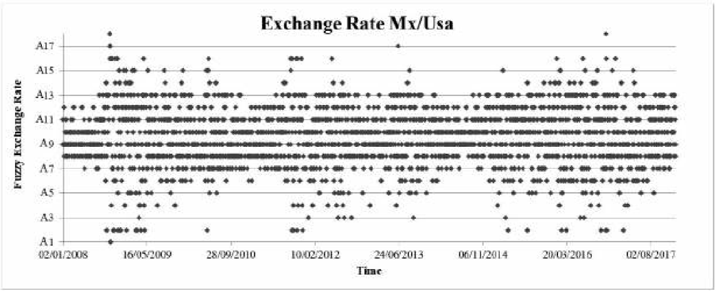
Source: Own elaboration in Excel with data from Banco of Mexico.
Figure 3 Fuzzy historical data of rate growth of the rate exchange MX/US
Table 1 Fuzzy relationship groups
| A1→A9,A17 |
| A2→A2,A5,A6,A7,A8,A9,A10,A11,A12,A13 |
| A3→A7,A8,A9,A10,A11,A12 |
| A4→A2,A3,A4,A5,A6,A7,A8,A9,A10,A11,A13 |
| A5→A2,A5,A7,A8,A9,A10,A12,A14,A16 |
| A6→A2,A3,A4,A5,A6,A7,A8,A9,A10,A11,A12,A13,A14,A16 |
| A7→A2,A3,A5,A6,A7,A8,A9,A10,A11,A12,A13,A14,A15,A16,A18, |
| A8→A2,A3,A5,A6,A7,A8,A9,A10,A11,A12,A13,A14,A15,A16,A17, |
| A9→A2,A3,A4,A5,A6,A7,A8,A9,A10,A11,A12,A13,A14,A15,A16 |
| A10→A2,A3,A4,A5,A6,A7,A8,A9,A10,A11,A12,A13,A14,A15,A16 |
| A11→A2,A3,A4,A5,A6,A7,A8,A9,A10,A11,A12,A13,A14,A15,A16 |
| A12→A2,A4,A5,A6,A7,A8,A9,A10,A11,A12,A13,A14,A15,A16 |
| A13→A2,A5,A6,A7,A8,A9,A10,A11,A12,A13,A14,A15,A16 |
| A14→A2,A5,A6,A7,A8,A9,A10,A11,A12,A13,A14 |
| A15→A7,A8,A9,A10,A11,A12,A13 |
| A16→A2,A4,A6,A7,A8,A9,A12,A13,A15,A16,A18 |
| A17→A1,A10,A16 |
| A18→ A1,A16 |
Source: Own elaboration with data from Banco of Mexico.
Step IV. Obtain the matrixes of possibility and relationships using the fuzzy time series generated in the previous stage.
We built the (14) and (15) matrices from the results of phase 3, using assumptions 1 and 2. Figure 3 shows the possible transition from one fuzzy subset to another. For example, if in the period F(t-1) the fuzzy exchange rate was A1 there is a probability of 50% of changing to the fuzzy subset A9 or A17. In the next period F(t), we face the same odds. We show the transition probabilities in (14).
On the other hand, (15) shows the fuzzy logic relationships between several subsets. Therefore, the 0's in the matrix indicates no relationship between the subsets, and 1's indicates a fuzzy logic relationship. It is important to stress that the reader must read the matrix in rows, from left to right.
As the reader may see, there is an intense concentration of the subset A7 to A12 oscillating between A2 and A16. In this idea, A7, A8, A9, A10, A11 and A12 can be understood as attraction states (Tsaur, 2012).
For A1, A2, A3, A4, A5 and A6, these are the fuzzy subsets generated by good news, because they cause an appreciation of the currency, in the same manner, A13, A14, A15, A16, A17 and A18 are the ones caused by bad news, they produce a depreciation of the exchange rate.
The first relevant result is that the methodology of the fuzzy time series provides better visualization of the exchange rate uncertainty because it identifies the appreciation and depreciation patterns in a graphical form.
A preliminary conclusion of this research is that the phenomena that profoundly impact on the behaviour of the exchange rate are transitory because fuzzy sets show a reversion to the state of attraction once the impact decreases.
Step V. Define the "If-Then" rules in the fuzzy process or define the first and second fuzzy rules to perform the defuzzification of the time series. Until this point, all the databases obtained are saved and combined with the results of the next step.
Figure 4 shows the fuzzy volatility areas, specifically denoting the possibility distribution of the 18 fuzzy subsets of the exchange rate. Each of the subsets is understood to have a certain level of possibility of transition to another fuzzy subset measured by an associated probability. For example, the area of A8 is the triangular membership function and it is composed by the transition probabilities from A8 to the other 18 fuzzy subsets, the sum of all probabilities in A8 is 1. The probabilities associated to each fuzzy subset can be seen in the matrix (14).
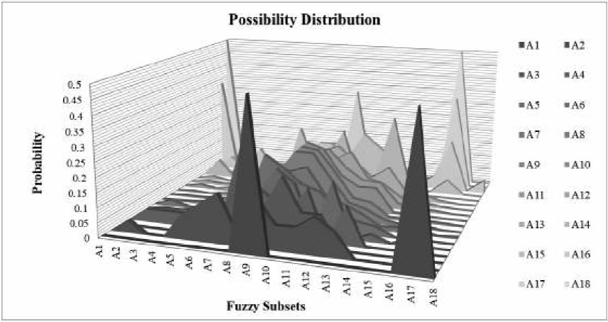
Source: Own elaboration in Excel with data from Banco of Mexico.
Figure 4 Possibility distribution of fuzzy subsets of the exchange rate MX/US
Step VI. Estimate the Fuzzy ARIMA Model by the Tseng et al. (2001) or Tanaka et al. (1982) methodology to identify the fuzzy subset associated with each forecast.
We described the analysis of the fuzzy time series in the previous stages using the fuzzy ARIMA model. We showed three predictions, one from the traditional ARIMA, other for the high ARIMA, and the third for the low ARIMA (see Table 5), and whereby we associate the fuzzy subset with each forecast using the step III method.
Table 3 presents the fuzzy parameters of the Fuzzy ARIMA model using Tanaka's estimation methodology. We categorize the parameters into three points of the triangular membership function. The β-ARIMA is the mean estimation; the high forecast gives the β-Upper while the β-Lower represents the low prediction. In this case, C is the width of the triangle membership function.
Table 3 Triangular fuzzy parameters of the Tanaka's model
| Lag | β-ARIMA | β-Upper | β-Lower | C |
|---|---|---|---|---|
| AR (1) | -0.5504*** | 0.00018 | -1.10110 | 0.55064 |
| AR (2) | 0.06132*** | 0.12329 | -0.00065 | 0.06197 |
| AR (3) | -0.0471*** | 0.00025 | -0.09459 | 0.04742 |
| AR (4) | -0.6149*** | 0.00031 | -1.23030 | 0.61530 |
| MA (5) | 0.6129*** | 1.22593 | 0.00000 | 0.61296 |
| MA (6) | 0.5461*** | 1.09464 | -0.00227 | 0.54846 |
| MA (7) | 0.0478*** | 0.09706 | -0.00131 | 0.04918 |
Source: Own elaboration in Excel with data from Banco of Mexico.
Using the Tanaka's methodology (5) we can create a triangular membership function for the AR(1) where the mean parameter is -0.5504, the upper is 0.34650, the lower is -1.44742, and the width is 0.89697, see annexe in figure A8.
We use bootstrap to generate ten thousand parameters for the high and low point of the function. We estimated the points that correspond to the one that solves the linear programming problem (5). The results showed that the set of high and low parameters include the optimal estimate, and also, the distribution of the coefficients for Tanaka's methodology follows a normal distribution. The parameters in Table 4 illustrate the estimation of fuzzy ARIMA through the Tseng's methodology; the interpretation and results are as described above.
Table 4 Triangular fuzzy parameters of the Tseng's model
| Lag | β-ARIMA | β-Upper | β-Lower | C |
|---|---|---|---|---|
| AR (1) | -0.5504*** | 0.34650 | -1.44742 | 0.89697 |
| AR (2) | 0.0613*** | 1.01079 | -0.88816 | 0.94948 |
| AR (3) | -0.0471*** | 0.70908 | -0.80341 | 0.75625 |
| AR (4) | -0.6149*** | -0.30054 | -0.92944 | 0.31445 |
| MA (1) | 0.6129*** | 1.40569 | -0.17976 | 0.79273 |
| MA (4) | 0.5461*** | 1.34047 | -0.24810 | 0.79429 |
| MA (6) | 0.0478*** | 0.54796 | -0.45221 | 0.50009 |
Source: Own elaboration in Excel with data from Banco of Mexico.
Step VI. Defuzzification.
In this step, We perform the association of the databases obtained in the previous steps and the combination of the fuzzy ARIMA model and the fuzzy time series theory. This step's goal is to build a forecast for the hybrid FTS-Fuzzy ARIMA model. Step VI shows the forecasts associated with the FTS-Fuzzy ARIMA model for the Mexican peso against the US dollar exchange rate.
Figure 5 illustrates the forecast for the proposed fuzzy FTS ARIMA model, based on Tanaka's methodology (grey line), and the actual exchange rate's yield (black line). The estimated values provide a better approximation of the analyzed time series compared to the results of the models presented in table 5 in the annexes.
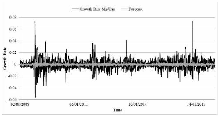
Source: Own elaboration in Excel with data from Banco of Mexico.
Figure 5 Forecast of FTS-fuzzy ARIMA Tanaka's model
Figure 6 depicts the forecast of the proposed fuzzy ARIMA FTS model, based on Tseng's methodology (light grey line) and the exchange rate yield (black line). The predicted values represent a better approximation for the time series analyzed in comparison to the results obtained from the models presented in Table 5.
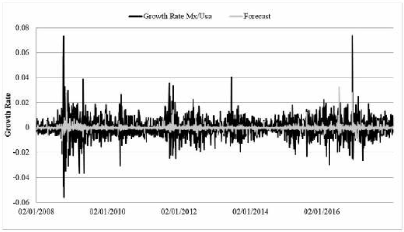
Source: Own elaboration in Excel with data from Banco of Mexico.
Figure 6 Forecast of FTS-fuzzy ARIMA Tseng's model
Table 5 In-Sample test
| Model\Statistic | Mean Absolute Deviation |
Root Mean Squared Error |
Log-likelihood | Jarque-Bera |
|---|---|---|---|---|
| ARIMA (4, 1, 6) | 0.005304 | 0.007714 | 8624.435 | 13063.41 |
| PARCH (1,1) | 0.005286 | 0.007748 | 8613.304 | 14637.83 |
| E-GARCH (1, 1) | 0.005279 | 0.007742 | 8615.262 | 15207.22 |
| Chen’s methodology | 0.013173 | 0.018420 | 6980.383 | 32712.22 |
| High Fuzzy ARIMA Tseng’s | 0.014248 | 0.020340 | 6201.501 | 19112.40 |
| Low Fuzzy ARIMA Tseng’s | 0.014330 | 0.020292 | 6212.230 | 6846.773 |
| High Fuzzy ARIMA Tanaka’s | 0.010308 | 0.014741 | 7003.695 | 12169.23 |
| Low Fuzzy ARIMA Tanaka’s | 0.010454 | 0.014715 | 7012.422 | 5165.949 |
| FTS-Fuzzy ARIMA Tseng’s | 0.005198 | 0.007595 | 8663.060 | 9931.244 |
| FTS-Fuzzy ARIMA Tanaka’s | 0.005156 | 0.007915 | 8559.667 | 101826.2 |
Source: Own elaboration in Excel with data from Banco of Mexico.
Table 5 also shows the in-sample results for the four efficiency measurements performed to verify our result's accuracy tests; the tests were: Mean Absolute Deviation, Root Mean Squared Error, Log-likelihood, and Jarque-Bera normality test. As the reader may see, the main result of all these measures is that models based on fuzzy theory present the best accuracy values for each test.
In the case of the Mean Absolute Deviation test, the best model was FTS-Fuzzy ARIMA (Tanaka's model) with an error 0.0012 points smaller the second-best performance. For the Root Mean Squared Error and the Maximum likelihood measurements, the model best model is the FTS-Fuzzy ARIMA (Tseng's model). Finally, the Jarque-Bera test reveals non-normal errors.
We show the out-of-sample forecast in table 6. On that table, we provide empirical evidence of the better performance of fuzzy-based models when compared to the traditional methods. Notably, the mean percentage daily error indicates that the FTS-Fuzzy ARIMA (the paper's model) is the one that best fits the exchange rate volatility.
Table 6 Out-Sample test
| Model\Test | Mean Percentage Daily Error | ||
|---|---|---|---|
| 1 day | 5 days | 10 days | |
| ARIMA | 0.4172% | 0.6199% | 0.4782% |
| PARCH | 0.3388% | 0.6076% | 0.4656% |
| E-GARCH | 0.3884% | 0.6077% | 0.4662% |
| Chen’s methodology | 0.8452% | 0.3851% | 1.3843% |
| FTS-Fuzzy ARIMA Tseng’s | 0.2719% | 0.5440% | 0.4488% |
| FTS-Fuzzy ARIMA Tanaka’s | 0.5814% | 0.5694% | 0.4714% |
Source: Own elaboration in Excel with data from Banco of Mexico.
The main difference between the models in table 6 and table 5 is that the Fuzzy-ARIMA method can not provide out-of-sample values because it does not produce a crisp forecast. It provides a prediction interval that we show in Figure 7, sections e.1 and e.2.

Figure 7 presents the out-of-sample forecasts. Section one (left side) shows the forecast for each model and compares it with the real data, while section 2 (right side) contains the graphs corresponding to the percentage evolution of the errors.
For instance, section f.1, (light grey), shows the out-of-sample forecast from FTS-Fuzzy ARIMA (Tseng's model) compared to the real volatility of the exchange rate (black line). Section f.2 shows the error's evolution throughout the study period. Remarkably, the FTS-ARIMA (Tseng's methodology) shows a stable deviation smaller than 1% from the actual value. Its result is significantly better than other models (section a.2, b.2, c.2 and d.2) because its result does not lose efficiency as the variable evolves.
Finally, the results presented in this section support the hypothesis and complement the objective of the research. We provided empirical evidence of a better forecast by a fuzzy time series models. We also showed that our model outperforms the Tseng's or Tanaka's FTS-ARIMA.
Conclusions
This paper's main conclusion is that fuzzy time series models can better estimate the behavior of variables characterized by high volatility, such as the exchange rate. We found that fuzzy theory improves the analysis and prediction when compared to traditional econometric models.
We also showed that the two models proposed in this paper outperform traditional models in high volatility environments, such as the MXP/USD exchange rate, both in out-of-sample and in-sample accuracy tests. Therefore, they provide more accurate forecasts for economic agents.
Along with the paper, we described the design and development of the FTS-Fuzzy ARIMA model and applied it to de MXP/USD yield. The proposed method produced better in-sample and out-sample forecast, even in high volatility environments. Our forecasts outperformed the traditional ARIMA, EGARCH and PARCH models.
It is important to stress that the fuzzy logic was successful in identifying time-series process volatility clusters or regime changes. The fuzzy methodology also mitigates the effect of error propagation in the out-sample exercises.
This research provides a new methodology to forecast the behavior of the exchange rate with higher precision, thereby contributing to the effort to improve forecasting techniques in support of decision making by economic agents in Mexico.

