


Serviços Personalizados
Journal
Artigo
 texto em
  Inglês (pdf)
 Artigo em XML
 Referências do artigo
 Enviar este artigo por email
Indicadores
-
 Citado por SciELO
 -
 Acessos
Links relacionados
-
 Similares em
SciELO
Similares em
SciELO
Compartilhar

 Permalink
Contaduría y administración
versão impressa ISSN 0186-1042
Contad. Adm vol.65 no.2 Ciudad de México Abr./Jun. 2020 Epub 09-Dez-2020
https://doi.org/10.22201/fca.24488410e.2020.1900
Articles
Impact of the introduction of the yellow corn futures contract on spot price volatility: Evidence from MexDer
1 Instituto Tecnológico y de Estudios Superiores de Monterrey, EGADE Business School, México
In October of 2012 the authorities of the Mexican Derivatives Exchange introduced the Yellow Corn Futures Contract in order to provide a more flexible mechanism of hedging to Mexican producers, given that this contract will be traded in Mexican Pesos and will be of 25 metric tons. On the other hand, it is also expected that this futures contract to contribute to volatility reduction of yellow corn in the spot market. Employing GARCH models, robust evidence is found to express that once the Futures Contract started operating the price volatility of this grain, in the spot market, was reduced.
JEL code: G14; G15; G18; G23; G28; G32
Keywords: Futures contracts; Yellow corn; Volatility; ARCH and GARCH models; Time series analysis
En Octubre del 2012 se introdujo el Futuro del Maíz Amarillo en el Mercado Mexicano de Derivados. Las autoridades del Sistema Financiero Mexicano esperan que: a) sea un instrumento de cobertura más apropiado para los productores mexicanos, dado que se opera en pesos y cada contrato es por 25 toneladas; b) su introducción contribuya en la disminución de la volatilidad en el mercado físico del maíz. Mediante el uso de estructuras GARCH, los resultados proporcionan evidencia robusta para afirmar que hubo una disminución en la volatilidad del precio físico del maíz amarillo, una vez que el contrato futuro fue introducido.
Código JEL: G14; G15; G18; G23; G28; G32
Palabras clave: Contratos futuros; Maíz amarillo; Volatilidad; Modelos ARCH y GARCH; Análisis de series de tiempo
Introduction
Derivative instruments emerged as a way of hedging risks during periods of high volatility in the prices of some primary inputs such as grains, copper, steel, gold, oil, and meat, among others. These inputs are currently used as a hedging mechanism for exchange rates, stock prices, and interest rates, among other financial assets, within what is known as Risk Management.
Speculators also use derivative instruments to obtain returns for selling or buying an asset, given certain expectations about the future behavior of the asset underlying the derivative. On the other hand, although challenging to realize in practice due to transaction costs and market efficiency, derivative instruments can be used for arbitrage. According to Tsetsekos and Varangis (2000), the first derivative instrument was an agricultural contract introduced in 1859 in the Chicago Board of Trade. This contract illustrated the importance of the field in the economic development of the United States. Later, in 1878, contracts on non-precious metals were created at the London Metal Exchange, and in the 1960s, on foreign exchange. It is worth mentioning that the use of derivative instruments was questioned because of their role in the 2008 housing crisis.
On the one hand, the abuse in the use of these instruments was a consequence of the lack of regulation of the corresponding entities and, on the other, the lack of transparency with which many of the organizations that used these financial instruments to speculate operated. Despite the above, there should be recognition for the role that derivatives play in the financial planning of organizations as they are appropriate mechanisms to hedge exchange rates, interest rates, and variations in the prices of important inputs in the productive processes of many companies and many industrial activities (natural gas, copper, steel, and agricultural products, among many others). However, there is information, as described below, that indicates that the participation of speculators can cause an increase in the volatility of the spot market.
One of the main benefits of derivative instruments is that they make it possible to take positions in the underlying asset, without actually being in possession of it. The above undoubtedly promotes proper risk management for organizations and for the economy in general, not to mention the vital role they play in the process of price formation of the underlying assets and the efficiency of the markets. Despite these benefits, some currents of thought claim that derivative instruments cause greater volatility in the markets since, in order for derivatives to function as hedging mechanisms, there must be a sufficient number of speculators taking positions contrary to those of the entities that wish to be covered. Many market participants interpret the above as a legal way to make bets, although the significant role that speculators play in market liquidity is undeniable. Scholars of the subject, through theoretical postulates and empirical evidence, have provided elements to affirm that the formally established derivative markets constitute, on the one hand, an appropriate hedge mechanism and, on the other, a mechanism of stabilization in the physical prices of the underlying assets of the instruments. With the introduction of futures contracts, the expectation is that, in addition to the hedge source it represents, there will be a decrease in the volatility of the changes in the prices of the underlying asset in the spot market. It is clear then that, in the case of the introduction of the Yellow Corn Futures Contract in the MexDer, the authorities of the Mexican Financial System expect that it will contribute to the price formation process and a decrease in volatility in the physical market of this grain. Additionally, it will facilitate the hedging process for Mexican producers, since it will be quoted in Mexican pesos and have a volume of 25 metric tons, unlike the Yellow Corn Futures Contract in the Chicago market, quoted in dollars and with a size of 5,000 bushels (127 metric tons).
The expectation of the Mexican Financial System authorities is supported by various theoretical postulates established by academics, among which the following stand out: a) the fact that the positions in the derivatives market increase, as a consequence of the low transaction costs - compared to those of the capital market - can propitiate a higher flow of information in the capital market and at the same time translate into greater liquidity, which would cause a decrease in the volatility of the capital market; b) the futures markets tend to increase the quality and quantity of information in the capital markets which would tend to decrease their volatility; (c) derivatives markets improve the efficiency of incomplete capital markets by increasing investment opportunities for participants; (d) the introduction of futures contracts can improve information efficiency by reducing asymmetries; (e) futures markets encourage a more efficient flow of information and consequently reduce the perceived variance in spot market futures prices.
Given the above, this article evaluates the impact that the introduction of the yellow corn futures contract in the Mexican Derivatives Market (MexDer) had on the volatility of the physical price of the grain. In order to achieve this evaluation, the stochastic dynamics of the percentage variations of the price of corn were modeled using an Autoregressive and Moving Average (ARMA) structure and a Vector Autoregressive (VAR) model to subsequently model the volatility through GARCH structures. The results obtained demonstrate that there is a significant decrease in the volatility of the physical price of grain after the implementation of the futures contract in the MexDer.
Presently, the Mexican Derivatives Market (MexDer) is working on the design of a futures contract for electricity prices, so the results of this research could provide elements to evaluate the feasibility of implementing this instrument. Then there is the further challenge of evaluating the possibility of implementing a derivatives market for agricultural products in Mexico, because of the significance that this sector has for the country. The rest of the article consists of four sections: a) Literature Review; b) Empirical Analysis; c) Results; and d) Conclusions.
Review of the Literature
Figlewski (1981) mentions that the introduction of futures contracts can increase the efficiency of the markets and smooth the variations in the prices of the underlying assets since, through the futures markets, the risk can be distributed among all the speculators and reduced for the entities that take hedging positions. This risk transfer can improve the functioning of the spot market as it reduces the need to incorporate a risk premium for variations in the prices of the products traded. On the other hand, futures markets increase the efficiency of the markets through all the information analyzed to estimate the future values of the assets considered, based on the information available. Simpson and Ireland (1985) studied the impact of Treasury Bond futures contracts on the volatility of returns in the spot market. Their results reveal that futures contracts decrease volatility in the spot market initially, but volatility increases as the volume traded in the futures market increases.
Dennis and Sim (1999) studied the impact that the introduction of stock futures contracts on the Sydney Futures Market had on spot price volatility. Their findings indicate that the impact on stock market volatility was virtually zero.
Rahman (2001) studied the introduction of derivative instruments on the Dow Jones Industrial Average index and their impact on the spot price of the shares that it lists. His findings exhibit that there were no structural changes in the conditional volatility of the prices of the shares that make up the index.
Debasish (2009) studies the impact of the introduction of the Nifty Index futures contract on the volatility of the index price in the spot market (National Stock Exchange). The results obtained demonstrate that there is no structural change in the volatility of the index price in the stock market.
Karathanassis and Sogiakas (2010) recount the theoretical assumptions that academics such as Cox, Friedman, and Ross, among others, make about the possible consequences in the spot market from the introduction of new derivative instruments. Among the most relevant, the authors highlight that where there could be opportunities for arbitrage, as a result of some distortion between the spot market and the derivatives market, the participants of both markets would be responsible for restoring the conditions of equilibrium. Therefore, it would not be possible to make abnormal gains consistently over time, provided that the markets are efficient. In view of the above, the expectation is that there would be no significant impact on the volatility of the spot market given the introduction of a new derivative instrument.
On the other hand, the authors of this article also present other postulates, from different perspectives, in which they establish that: a) the fact that the positions in the derivatives market increase, as a result of the low transaction costs-compared with those of the capital market-can propitiate a greater flow of information in the capital market and at the same time translate into greater liquidity, which would cause a decrease in the volatility of the capital market; b) the futures markets tend to increase the quality and quantity of information in the capital markets which would tend to decrease their volatility; (c) derivatives markets improve the efficiency of incomplete capital markets by increasing investment opportunities for participants; (d) the introduction of futures contracts can improve information efficiency by reducing asymmetries; (e) futures markets encourage a more efficient flow of information and consequently reduce the perceived variance in spot market futures prices.
Moreover, regarding empirical evidence, Karathanassis and Sogiakas (2010) review the critical findings in developed financial markets and find that for the United States, the United Kingdom, Switzerland, Germany, Japan, Spain, Italy, and Greece, the introduction of specific derivative instruments has stabilized the operation in the respective spot markets. Conversely, this same article mentions that other authors have found that the introduction of new derivative instruments has destabilized prices in the spot markets. These findings imply that the conclusions on the impact of the introduction of a derivative instrument on the volatility of the underlying asset are not conclusive.
According to Songwe (2011), the high volatility in recent years in the price of raw materials, exchange rates, and interest rates, has led to an increased use of derivatives. Proof of this is that derivative instruments have had the most significant growth in comparison to other financial instruments in the stock markets of developed countries. Songwe (2011) also points out that, specifically, futures contracts with underlying agricultural assets began to grow rapidly at the end of 2004. This growth was due not only to the increase and volatility in prices but also to the improvement in the trading infrastructure and an increase in the quality and speed of access to relevant information. The above led to an increase in the volume traded from US $13 trillion in 2003 to a volume of US $260 trillion in 2008.
In the same vein, Girardi (2012) highlights the importance and influence that derivative instruments have in the process of forming physical prices of some primary inputs. However, at the same time, Girardi questions the role that speculators have had in the very drastic fluctuations in the prices of some products such as corn, soybeans, wheat, and rice. Specifically, Girardi presents data on how the purchase of derivative instruments for these inputs grew between 2004 and 2008, which caused upward pressure on the physical price of these products. On the other hand, the author also mentions that at the end of 2008 and beginning of 2009, a very important sales process of these positions was registered, which contributed to the fall of physical prices and, consequently, to the increase of volatility. Girardi (2012), in an analysis for wheat, provides elements to affirm that these variations in the physical prices of this input, between 2004 and 2008, were not due to an increase in the demand or a decrease in the supply, nor that the fall in the prices, between 2008 and 2009, was due to a decrease in the demand or an increase in the supply. The above is explained based on the speculative positions taken in the most important derivatives markets of the world.
Conversely, Bohl and Stephan (2012) analyze the impact of agricultural commodity and energy futures on the physical price and find no compelling evidence that trading in futures contracts induces greater volatility in the prices of the products underlying the contracts.
The above has given rise to several debates related to the role that futures contracts play in distorting the physical prices of certain agricultural products, mainly due to the speculative process that takes place in the derivatives markets and the influence that such positions have on the physical prices of the generics underlying the contracts. On the other hand, Morgan, Rayner, and Vaillant (1999) give an account of the main findings obtained by several researchers on how the futures markets have contributed to the stabilization of the prices in the spot market, for several generic products in developed countries. In this same work, these authors also review how international futures markets have contributed to the process of price stabilization in the physical markets for specific essential food inputs in less developed countries that do not have a derivatives market.
In the same vein, Bernard, Greiner, and Semmler (2012) mention that every time a contract is executed in the forward market or a futures contract for agricultural products, it informs and influences the formation of prices in the spot market. Therefore, it makes sense to think about the influence that derivatives markets have on physical markets.
Spyrou (2005) analyzes the impact of the introduction of the Athens Stock Exchange index futures contract on spot price volatility. The results indicate that there was no change in the volatility of the index due to the introduction of this derivative. Vipu (2006) investigated the changes in the volatility of the Indian Stock Exchange, after the introduction of derivative instruments for the shares. The results reveal that there is a reduction in the conditional volatility of stock prices after the introduction of the derivative instruments. However, there is an increase in the unconditional volatility. This apparent contradiction is explained in terms of the increased correlation between stock prices caused by arbitrage in the spot market, which has led to many questions and debates about the role that derivatives have in the markets.
Bose (2008) mentions that the main functions of a futures market are to provide hedging mechanisms and influence price stabilization in the spot market. Floros and Vougas (2006) analyze the impact that the introduction of a stock index future had on the volatility of the Greek stock market and find that the volatility of a stock index for highly-securitized issuers (FTSE/ASE-20) decreases, while the volatility of an index for medium-securitized issuers (FTSE/ASE-Mid 40) increases. Perhaps these findings can be explained by the level of information generated around highly securitized issuers, which in general tends to be higher than that generated around medium-securitized issuers, as a result of the level of analysis carried out for both.
On the other hand, Ghosh (2011) analyzes the implications that could derive from a regulatory process in derivatives markets for generic products and, among others, highlights the significance of migrating to formally established derivatives markets to induce greater transparency and regulation of investor activity in these markets and thus avoid distortion of physical prices.
Chevallier, Le Pen, and Sévi (2011) studied the primary market of the European Union and analyzed the impact that the introduction of options had on the volatility of the instrument designed to mitigate pollutant emissions. Their results reveal that the introduction of financial options contributes to reducing volatility in the primary market. In the case of Mexico, Del Alto (2012) analyzed the impact that the introduction of the futures contract on the Prices and Quotations Index (Spanish: Índice de Precios y Cotizaciones, IPC) had on the volatility of the index in the stock market. He found that there is statistical evidence to affirm that there was a significant decrease in the volatility of the IPC after the introduction of the futures contract in the Mexican Derivatives Market.
Hayali (2014) studied the role of derivatives in the Mexican financial crisis of the 1990s. His results indicate that financial instruments had a significant influence on this crisis, as they had an immediate destabilizing effect on exchange rate volatility. This result is consistent with the currents of thought that claim that derivative instruments increase the volatility of the underlying assets as a result of the role played by speculators. This result has sparked a good deal of debate in various studies related to the role of derivative instruments in spot markets. For this reason, one of the objectives of this work is to understand the impact of these instruments in an emerging market like Mexico.
In this context, it is clear that one of the primary uses of derivative instruments, and particularly of futures contracts-in addition to contributing to the process of price stabilization in the physical market-is that of risk management, since it allows for the definition of hedging mechanisms against fluctuations in the price of the underlying assets. Regarding the fluctuations of white corn prices, Godínez (2007) analyzes the usefulness of using the US #2 yellow corn futures prices of the Chicago Exchange as an international hedging mechanism for producers and traders of white corn in Mexico. For this hedging to be relevant and useful, the future price must maintain leadership and causality over physical prices in Mexico. Through the Granger criterion of the Vector Autoregressive model and Causality tests, he finds that the hedging is not relevant. Concerning these findings, they may be a result of cross hedging (since variations in the price of white corn are hedged with a futures contract for yellow corn) done in dollars, which results in an additional risk factor for Mexican producers. In this sense and in accordance with the above, in the first instance, it is appropriate to introduce futures for yellow corn since when operating in Mexico the contracts will be defined in Mexican pesos and the size, of 25 tons, will be more in line with the needs of Mexican producers. The yellow corn futures contracts traded in Chicago are 5,000 bushels, equivalent to 127 tons, also traded in dollars, which triggers an additional risk factor.
Importance of corn in Mexico
According to the USDA (United States Department of Agriculture), worldwide, Mexico is the sixth largest corn producer after the United States, China, the European Union, Brazil, and Argentina. On the other hand, according to the Ministry of Agriculture, Livestock, Rural Development, Fisheries, and Food (Spanish: Secretaría de Agricultura, Ganadería, Desarrollo Rural, Pesca y Alimentación, SAGARPA), Mexico is the largest consumer of corn in the world and represents 11% of global demand. Each Mexican consumes, on average, 123 kg of corn per year, a figure far higher than the average annual per capita consumption in the world of almost 17 kg.
In Mexico, the SAGARPA, through the Agri-Food and Fisheries Information System (Spanish: Sistema de Información Agroalimentaria y Pesquera, SIAP), recognizes three types of corn, according to their use, although there are various forms of cultivation: a) fodder corn, used as cattle feed, especially for dairy cows; b) grain corn, of which the white and yellow varieties are recognized. White grain corn is used mainly for food, because of its high nutritional value, but oil and inputs for the manufacture of varnishes, paints, artificial rubbers, and soaps can also be obtained from it. Yellow corn grains are also used for human consumption in a wide variety of dishes. However, their primary destination is livestock feed and starch production; and (c) popping corn, especially for the production of popcorn. According to SIAP figures, in 2010, Mexico produced about 23.3 million metric tons of corn, of which approximately 21 million corresponded to white corn, 2 million to yellow corn, and the rest to other types of corn. From the above figures, it is possible to see that almost 99% of corn production in Mexico in 2010 was grain corn (white and yellow), and of the total grain corn produced, almost 10% was yellow corn.
On the other hand, according to the Agricultural Marketing Support and Services (Spanish: Apoyos y Servicios a la Comercialización Agropecuaria, ASERCA), another agency of SAGARPA, between 2012 and 2013, Mexico produced, on average, about 21.5 million tons of grain corn per year, of which about 1.8 million tons correspond to yellow corn. According to SAGARPA, annual production of yellow corn is enough to satisfy a large part of human consumption, but not all of it, so to meet this demand and that generated by animal and industrial use, Mexico has to import the grain. It is important to mention that imports of yellow corn have increased, and imports of approximately 8 million tons have been estimated for 2018, which will mean that about 80% of total consumption will be supplied from abroad if the level of production in Mexico remains stable. Currently, according to the World Bank, about 50% of the total consumption of yellow corn in Mexico is supplied by imports from other countries.
As a result of the role that futures contracts play in the process of stabilizing the prices of the underlying assets, given the relevance of corn in the diet of Mexicans, which places the country as the leading consumer of corn in the world, and due to the high level of variability that the price of this grain has had in the world, it is of interest to analyze the impact that the introduction of the Yellow Corn Futures Contract had on the volatility of the physical prices of this grain in Mexico.
Empirical Analysis
Given that the objective of this article is to analyze the impact that the introduction of the yellow corn futures had on the volatility of this grain in the spot market, GARCH models will be estimated to quantify the variation in volatility once the futures contract was introduced into the Mexican Derivatives Market. The following is a description of the data used and the methodology employed.
Data Description
In order to carry out the empirical analysis, this article used the quotations of yellow corn in the spot market, provided by Bloomberg. This source of information includes quotations from the Chicago Mercantile Exchange and quotations from Latin America, which are formed by a weighted average of the quotations of the primary producers in the region, which are, in order of importance, Brazil, Argentina, and Mexico. This work used the quotations of Latin America. The data are weekly, from January 2007 to June 2013, which gives a total of 336 observations, and are in Mexican Pesos (MXN) per metric ton. Also used were the quotations of white corn, in the spot market, provided by the Mexican Stock Exchange, through SIBOLSA. These data are also weekly, from January 2007 to June 2013, and are in US cents per bushel, which in the case of corn is equivalent to 25.4 kg. The above was done because, through cross hedging, positions in white corn can be hedged from futures contracts for yellow corn.
Methodology
In order to model the volatility of the change in the price of yellow corn and understand if there was an impact from the introduction of the futures contract of this grain in the MexDer, structures of the GARCH family (Generalized Autoregressive Conditionally Heteroscedasticity) will be estimated after modeling the variation structure of the change in the physical price of corn. First, the stochastic variation structure of the change in the physical price of the grain will be modeled and then the volatility.
In order to achieve the above and to increase the robustness of the analysis, models belonging to two families will be estimated: a) A VAR (Vector Autoregressive) for the change in the price of both types of corn together, and b) A model of the ARMA family (Autoregressive Moving Average) for the change in the price of yellow corn to model the dynamics of variation in the changes in the physical price of the grain. Once the models of both families have been estimated, the volatility for each of them will be modeled using GARCH structures with a qualitative variable as a regressor, related to the introduction of the Future of Yellow Corn in Mexico, in order to quantify its impact on price volatility in the spot market.
ARMA Models
Autoregressive and Moving Average Structures (or ARMA) are useful for modeling the stochastic dynamics of series variation over time by capturing how the past of a variable, as well as past elements of the financial and general business environment, affect it. Unlike a structural econometric model, an ARMA family model makes it possible to obtain, from the behavior of the series analyzed, relevant information that will make it possible to determine the shape of the model to be estimated. In general terms, an Autoregressive and Moving Averages model has the following form:
which is formally called an ARMA(p, q) model since it includes p lags of the variable to be modeled and q lags of the random component of the model, which in a certain way contains the elements of the environment that surround the phenomenon under study. The random component of the previous model, in the context of time series modeling, is commonly called white noise as a result of the statistical characteristics assumed for it:
It is important to emphasize that to estimate the model parameters it is necessary to meet conditions of second-order stationarity for the variable of interest. The conditions above are summarized in the fact that the roots resulting from solving the characteristic equation, both the Autoregressive part and the Moving Averages part, must be of a magnitude greater than one or, equivalently, the magnitude of the inverted characteristic roots must be contained within a unit circle. The above would mean that the older the lags, both of the variables to be modeled and of the random component of the model, the less incidence they will have on the present achievements of the variable studied. In general terms, this is the expectation when working with a time series.
In other words, and in the context of this article, it would make sense to think that both what happened with the price of corn, and what happened in the economic environment surrounding the formation of its price, two or three weeks ago, have more influence on the price that will be observed this week, than what happened 20 weeks ago.
Having estimated the ARMA model for the change in physical prices of yellow corn, their volatility will be modeled using GARCH structures, which are described later in this section.
VAR Models
It is possible to think of Vector Autoregressive models as a generalization of Autoregressive structures combined with structures of simultaneous equations, in which all the variables that make up the Vector are considered endogenous. For the study of the problem in this article, the Vector Autoregressive model comprises two variables, which are the change in the price of yellow corn and the change in the price of white corn, so that the Vector Autoregressive model will have the following structure:
The above approach implies that the aim is to determine whether it is possible to understand each variable as a function of the lags of the other variable, in addition to being modeled as a function of its lags (as would be the case with a purely Autoregressive structure). In other words, if the aim is to determine whether the lags of Y 2,t anticipate the variance dynamics of Y 1,t it would be necessary to prove the following hypothesis statistically:
A similar assumption would have to be made and tested to determine whether the lags in Y 1,t anticipate the stochastic variation dynamics of Y 2,t .
It is important to mention that it is necessary to comply with the principle of stationarity in the case of the variables that comprise the Vector Autoregressive model so that it can be adequately estimated. Later, depending on the estimated VAR, its volatility will be modeled, also using GARCH structures.
GARCH Models
According to Brooks (2008), the modeling and prediction of volatility in stock markets has been the subject of numerous theoretical and empirical investigations, given the importance of this concept in the financial sphere since it is a widely used measure of financial asset risk. Moreover, models to determine the Value at Risk (VaR) of a financial market or the same expression as Black-Scholes-Merton, to value options, require the estimation of the volatility of the asset under consideration.
Given the objective of this research, rather than estimating volatility at a given point in time, it is necessary to model it historically through an Autoregressive Structure of Conditional Heteroscedasticity to determine if there was a significant change in its structure, once the Yellow Corn Futures Contract was introduced into the MexDer. Previously, in this same section on the description of the methodology, it was mentioned that the random component, which appears in the models already described, has certain statistical properties and that, independently of the assumed probability distribution, the following can be considered:
In situations like the above, the principle of homoscedasticity is fulfilled since the variance of the random component is constant at all times. On the other hand, when the variance is not constant for every moment, there is heteroscedasticity. Bollerslev (1986) and Taylor (1986) independently developed the GARCH model, which is an extension of the ARCH model developed by Engle (1982). In a GARCH model, the variance structure of the random component is as follows:
Thus, according to the objective of this article, the structure to be modeled will be:
where the qualitative variable is
It is clear that, for volatility, this will be the structure to be estimated once the stochastic dynamics of the variation in price for yellow corn are modeled using the two models described above. Given that the objective of this article is to determine the impact that the introduction of the Yellow Corn Futures Contract in the MexDer had on the volatility of the change in the physical price of the grain, the analysis will be done by statistically testing the following set of hypotheses:
It is apparent that, if the null hypothesis is not rejected, there would be evidence to affirm that the introduction of the Yellow Corn Futures Contract in the MexDer did not have a significant impact on the volatility of the change in the physical price of the grain. On the other hand, if the null hypothesis is rejected, and depending on the sign of the point estimate, it is possible to think about the influence of the introduction of this derivative instrument on the increase or decrease of the volatility of the price of yellow corn in the spot market.
Results
Figure 1 illustrates price changes over time for both yellow corn in Latin America and white corn in Mexico. As mentioned above, the price of yellow corn is in MXN/Ton, and its reference axis is the left side. The price of white corn is in USD cents/Bushel, and its reference axis is the right side. This figure displays a considerable increase in the price of both types of corn, starting in the second half of 2008 and a period of apparent stability during 2009 and until the third quarter of 2010 to define an upward trend in the price of both types of corn from the last quarter of 2010.
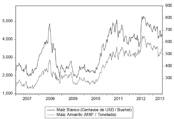
Source: own elaboration with data from Bloomberg and SIBOLSA
Figure 1 Yellow Corn and White Corn Price Variations
This figure demonstrates that the prices of both types of corn “move together,” so it is natural to think that the Pearson correlation coefficient between the prices of both types of corn is high (0.948732) and statistically significant. The high correlation between the prices of both types of corn facilitates cross-hedging, that is, that the variations in the price of white corn are hedged with the futures of yellow corn, a fundamental aspect in the case of Mexico given that 90% of the grain corn produced in this country is to white corn.
Instead of working directly with corn prices, a variable for both types of corn will be constructed. This variable corresponds to the weekly yield, determined on an ongoing basis, for someone with a long position in the physical market. It is also possible to think of this variable as the price growth rate or simply as a change in the physical price of both types of grain, in relative terms. With this in mind, it should be clear that the relationship between the price of week t and the price of week t-1 is given by P
t
= P
t◻1
Figure 2 illustrates the yield or growth rate of the price in the physical market, both for the quotation of white corn in Mexico and the quotation of yellow corn in Latin America.
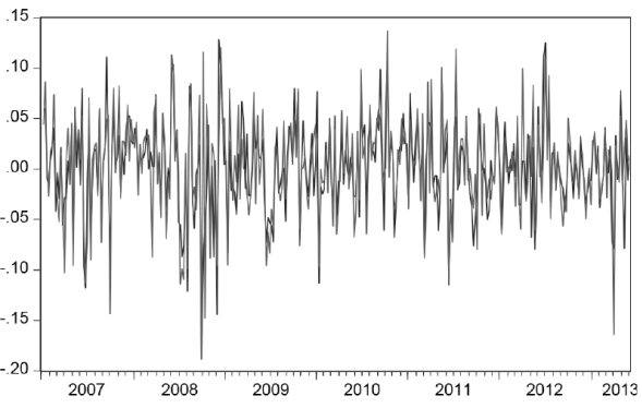
Source: own elaboration with data from Bloomberg and SIBOLSA
Figure 2 Yield of Yellow Corn and White Corn Quotations
The figure above demonstrates that the variation in yields, over time, for both types of corn is very similar. For these variables, the Pearson correlation coefficient is 0.773 and is statistically significant.
VAR Estimation
In addition to the methodology used to understand the dynamics of variation in the change of prices and thus model the volatility, it is also interesting to know the dynamics of variation in the yields of both types of corn, with the aim of understanding if the formation of the price of one type of corn anticipates the formation of the other, even more so when, in Mexico, the production of grain corn is fundamentally of white corn, as has been described previously. Before estimating the Vector Autoregressive, it is necessary to determine if the variables that make it up are stationary. To this end, the Dickey-Fuller Augmented Test, the Elliott-Rothenberg-Stock DF-GLS Test, and the Phillips-Perron Test will be carried out to verify if there are unitary roots, both in the yields of yellow corn and in those of white corn. Table 1 presents the results of the tests for yellow corn, where the Null Hypothesis establishes the existence of a unit root.
Table 1 Augmented Dickey-Fuller Test, Elliott-Rothenberg-Stock DF-GLS Test, and Phillips-Perron Test for yellow corn yields
| Dickey-Fuller Augmented Test | Elliott-Rothenberg-Stock DF-GLS Test | Phillips-Perron Test | |||
|---|---|---|---|---|---|
| Test Statistic | -16.63676 | Test Statistic | -13.834792 | Test Statistic | -16.6096 |
| Prob.* | 0 | Prob.* | 0 | Prob.* | 0 |
| Critical Test Values | Critical Test Values | Critical Test Values | |||
| 1% level | -3.449738 | 1% level | -2.572053 | 1% level | -3.44974 |
Source: own statistical analysis with data from Bloomberg
Table 1 demonstrates that all tests reject the existence of a unit root, which means that the dynamics of variation in yields or the rate of change in the price of yellow corn obeys a stationary process. In this same order of ideas, Table 2 presents the results of these same tests for the yields of white corn. The Null Hypothesis in the three tests establishes the existence of a unitary root.
Table 2 Augmented de Dickey-Fuller Test, Elliott-Rothenberg-Stock DF-GLS Test, and Phillips-Perron Test for white corn yields
| Augmented Dickey-Fuller Test | Elliott-Rothenberg-Stock DF-GLS Test | Phillips-Perron Test | |||
|---|---|---|---|---|---|
| Test Statistic | -16.63676 | Test Statistic | -13.834792 | Test Statistic | -16.6096 |
| Prob.* | 0 | Prob.* | 0 | Prob.* | 0 |
| Critical Test Values | Critical Test Values | Critical Test Values | |||
| 1% level | -3.449738 | 1% level | -2.572053 | 1% level | -3.44974 |
| 5% level | -2.869978 | 5% level | -1.941796 | 5% level | -2.86998 |
| 10% level | -2.571335 | 10% level | -1.61605 | 10% level | -2.57134 |
Source: own statistical analysis with data from SIBOLSA
Table 2 reveals that, in terms of the results of the three tests, the yields of white corn also obey a stationary process. Therefore, the VAR can be estimated directly, where any transformation for these two variables is unnecessary.
First, a Vector Autoregressive model with two lags will be arbitrarily estimated for the variables on the right to identify the optimal number of lags to include in the VAR. Table 3 presents the results of the selection process of the number of lags for the variables that comprise the Vector.
Table 3 Selection criteria for the number of lags for VAR variables
| Lag | LogL | FPE (Final Prediction Error) | AIC (Akaike Information Criterion) | SC (Schwarz Information Criterion) | HQ (Hannan-Quinn Information Criterion) |
|---|---|---|---|---|---|
|
|
|
|
|
|
|
VAR Lag Selection
Endogenous variables: RMAMARILLO RMBLANCO
Sample: 1/01/2007 6/03/2013
* indicates the optimal number of lags for each criterion
Source: own statistical analysis with data from Bloomberg and SIBOLSA
From the table above, and in terms of the different selection criteria, it is clear that the Vector Autoregressive model must contain a lag in each variable on the right, so for this case, the structure of the VAR is as follows:
In this case Y1,t represents the yield of yellow corn and Y2,t represents the yield of white corn, so the Vector Autoregressive model implies that the dynamics of yield variation for each type of corn is a function of a time lag in itself and a time lag in the other type of corn.
Table 4 presents the estimate of the VAR composed of these two variables and with a lag in each of them on the right side of the vector.
Table 4 Estimation of the VAR for the yields of yellow and white corn
| RMAMARILLO | RMBLANCO | |
|---|---|---|
| RMAMARILLO(-1) |
|
|
| RMBLANCO(-1) |
|
|
| C |
|
|
Estimation of the Vector Autoregressive model
Sample (adjusted): 1/15/2007 6/03/2013
Standard Errors in ( ) and t-statistic in [ ]
Source: own statistical analysis with data from Bloomberg and SIBOLSA
Based on the estimated VAR, the Granger Causality Test will be applied to determine if the yield variations of both types of corn anticipate the other. For this particular model, the structure is:
The Granger Causality Tests are equivalent to statistically verifying the fulfillment of the following hypotheses:
For the first set of hypotheses, this means that if α 11=0 is rejected, there would be elements to affirm that the yields of white corn anticipate the yields of yellow corn. On the other hand, for the second set of hypotheses, if α 21=0 is rejected, then there would be evidence to state that the yields of yellow corn anticipate the yields of white corn. Table 5 includes the results of the Granger causality tests for the previously estimated VAR.
Table 5 Granger VAR Causality Tests for Yields of Both Types of Corn
| Dependent Variable: RMAMARILLO | |||
| Chi-Squared | GL | Prob. | |
| RMBLANCO | 29.08965 | 1 | 0.0000 |
| Dependent Variable: RMBLANCO | |||
| Chi-Squared | GL | Prob. | |
| RMAMARILLO | 2.492587 | 1 | 0.1144 |
VAR Granger Causality Test
Sample: 1/01/2007 6/03/2013
Source: own statistical analysis with data from Bloomberg and SIBOLSA
The results of Table 5 indicate that for the first set of hypotheses α 11=0 is rejected, which means that the order 1 lag in white corn yields is significant in the yellow corn equation, implying that white corn yields anticipate the stochastic dynamics of yellow corn yields. A different way to interpret these results is that the formation of the price of white corn anticipates the formation of the price of yellow corn. For the second set of hypotheses, the situation is different. From the results presented in this same table, the conclusion is that the estimate α 21 is not statistically significant. Therefore, there are elements to affirm that the yields of yellow corn do not anticipate the yields of white corn. The aforementioned is consistent in terms of the percentages produced in Mexico for each of these two types of corn, as described in the literature review section. In other words, it is understandable that when 90% of corn produced in Mexico is white and 10% is yellow, there is influence or anticipation in the formation of the price of the first type of corn over the second. The breakdown of the estimated VAR variance confirms these results in Figure 3.
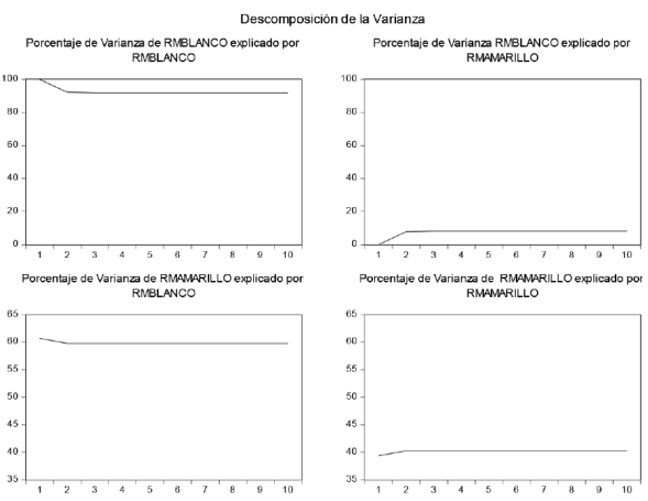
Source: own statistical analysis with data from Bloomberg and SIBOLSA
Figure 3 Breakdown of the variance of the VAR for the yields of yellow and white corn
Based on the previous results, which included statistical evidence to affirm that the yields of white corn anticipate the yields of yellow corn, but not the contrary, the first component of the VAR will be analyzed:
The above means that the ARCH test will be carried out and, where applicable, some GARCH structures will be modeled for the first VAR equation, which corresponds to the yields of yellow corn as a function of the order 1 lags of the yields of white corn. Table 6 displays the ARCH test for the residuals of the first VAR equation. It is worth noting that the null hypothesis in this test establishes stability in the variance of the residuals.
Table 6 ARCH test for residual yellow corn yields of VAR
| F-statistic | 6.584598 | Prob. F(4,326) | 0.0000 | |
| Obs*R-Squared | 24.74328 | Prob. Chi-squared (4) | 0.0001 | |
| Test equation: | ||||
| Dependent Variable: RESID^2 | ||||
| Sample (adjusted): 2/12/2007 6/03/2013 | ||||
| Variable | Coefficient | Standard Error | t-statistic | Prob. |
| C | 0.000703 | 0.000158 | 4.432433 | 0.0000 |
| RESID^2(-1) | 0.233211 | 0.055375 | 4.211458 | 0.0000 |
| RESID^2(-2) | 0.107156 | 0.056763 | 1.887788 | 0.0599 |
| RESID^2(-3) | -0.064936 | 0.056781 | -1.143617 | 0.2536 |
| RESID^2(-4) | 0.014123 | 0.055871 | 0.252771 | 0.8006 |
Source: own statistical analysis with data from Bloomberg and SIBOLSA
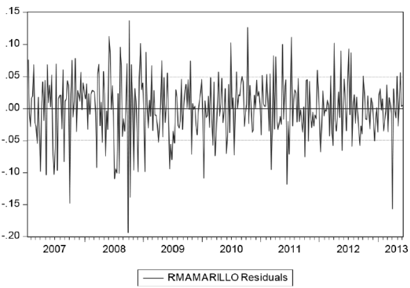
In terms of the results presented in the table above, it can be concluded from the test statistics that the hypothesis of stability in volatility is rejected, meaning that over time the variance is not stable. Figure 3 can corroborate this, and it presents the estimated model residuals over time.
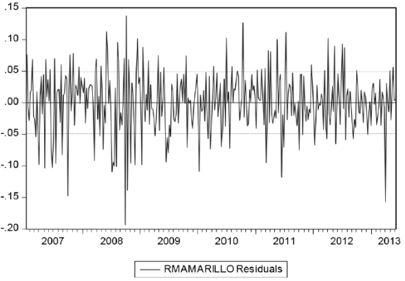
Source: own elaboration with data from Bloomberg and SIBOLSA
Figure 4 Residuals of VAR yellow corn yields
Based on the results obtained from the ARCH test, the necessary elements to proceed with the estimation of the GARCH model for the volatility of yellow corn yields are in place. It is important to remember that the general structure of the model for volatility is:
in which the variable FUTMAIZ is a qualitative variable that takes the value of zero on the dates when there was no futures contract for yellow corn in the MexDer and takes the value of one of the dates when this derivative instrument was already traded in the Mexican Derivatives Market. Table 7 presents the correlogram of the squared residuals of the first equation of the VAR to propose appropriate orders in the estimation of the GARCH structures. It seems that GARCH structures of up to order (2.2) would be appropriate.
Table 7 Correlogram of the squared residuals of VAR yellow corn yields
| Autocorrelation | Partial Autocorrelation | AC | ACP | Q-statistic | Prob | |
|---|---|---|---|---|---|---|
| .|** | | .|** | | 1 | 0.250 | 0.250 | 21.133 | 0.000 |
| .|* | | .|* | | 2 | 0.152 | 0.095 | 28.922 | 0.000 |
| .|. | | .|. | | 3 | 0.001 | -0.061 | 28.922 | 0.000 |
| .|. | | .|. | | 4 | 0.015 | 0.015 | 28.998 | 0.000 |
| .|. | | .|. | | 5 | 0.028 | 0.033 | 29.268 | 0.000 |
| .| | | .| | | 6 | 0.148 | 0.142 | 36.810 | 0.000 |
| .|. | | |. | | 7 | 0.008 | -0.070 | 36.834 | 0.000 |
| .|. | | .|. | | 8 | 0.011 | -0.013 | 36.874 | 0.000 |
| .|. | | .| | | 9 | 0.054 | 0.081 | 37.885 | 0.000 |
| .|. | | .|. | | 10 | -0.018 | -0.053 | 37.999 | 0.000 |
| .|. | | .|. | | 11 | 0.016 | 0.011 | 38.090 | 0.000 |
| .|. | | .|. | | 12 | 0.013 | -0.001 | 38.151 | 0.000 |
| .|. | | .|. | | 13 | 0.053 | 0.062 | 39.152 | 0.000 |
| .|. | | .|. | | 14 | 0.034 | 0.009 | 39.569 | 0.000 |
| .|. | | .|. | | 15 | 0.040 | -0.005 | 40.135 | 0.000 |
| .|. | | .|. | | 16 | -0.008 | -0.003 | 40.157 | 0.001 |
| .|. | | .|. | | 17 | -0.027 | -0.034 | 40.423 | 0.001 |
| .|. | | .|. | | 18 | -0.012 | 0.001 | 40.474 | 0.002 |
Sample: 1/08/2007 6/03/2013
Source: own elaboration with data from Bloomberg and SIBOLSA
Table 8a presents the results of the estimated GARCH model (1.2), whose order was selected because it optimizes the selection criteria of Akaike, Schwarz, and Hannan-Quinn.
Table 8a Estimation of the GARCH (1.2) model for the volatility of VAR yellow corn yields
| Dependent Variable: RMAMARILLO | ||||
|
| ||||
| Variance Equation | ||||
| Variable | Coefficient | Standard Error | t-statistic | Prob. |
| C | 0.000554 | 9.05E-05 | 6.123148 | 0.0000 |
| RESID(-1)^2 | 0.345375 | 0.084524 | 4.086104 | 0.0000 |
| GARCH(-1) | 0.314431 | 0.155564 | 2.021233 | 0.0433 |
| GARCH(-2) | -0.164139 | 0.096325 | -1.704011 | 0.0884 |
| FUTMAIZ | -0.000184 | 9.60E-05 | -1.918993 | 0.0550 |
Source: own statistical analysis with data from Bloomberg and SIBOLSA
Table 8b presents the results of the TARCH model (1.2), whose order was selected because it minimizes the selection criteria of Akaike, Schwarz, and Hannan-Quinn.
Table 8b Estimation of the TARCH (1.2) Model, with a threshold order of 1, for the volatility of the VAR yellow corn yields
| Dependent Variable: RMAMARILLO | ||||
|
| ||||
| Variance Equation | ||||
| Variable | Coefficient | Standard Error | t-statistic | Prob. |
|
|
|
|
|
|
Source: own statistical analysis with data from Bloomberg and SIBOLSA
From the previous tables, in the estimated GARCH structure, the qualitative variable has a negative sign and is statistically significant when considering a significance of 10%. This means that there is evidence to affirm that, after the introduction of the yellow corn future in the MexDer, there was a statistically significant decrease in the volatility of yellow corn yields of 1.36% when measured in terms of standard deviation
Estimation of the ARMA structure
It has been determined, in the process of estimating the VAR, that the yields or growth rates in the prices of yellow corn are governed by a stationary process which allows them to be modeled, without the need for any transformation, using structures from the ARMA family. After a process of identification and optimization of the information criteria of Akaike, Schwarz, and Hannan-Quinn, an ARMA structure (4.4) was chosen for the yields of yellow corn. This means that, if Yt represents the yields of yellow corn, then the structure to be estimated has the following form:
The estimation of the previous model, obtained from the available history, is illustrated in Table 9.
Table 9 ARMA structure estimate (4.4) for yellow corn yields
| Dependent Variable: RMAMARILLO | ||||
| Sample (adjusted) 2/05/2007 6/03/2013 | ||||
| Variable | Coefficient | Standard Error | t-statistic | Prob. |
|
|
|
|
|
|
| Inverted AR Roots | .91-.31i | .91+.31i | -.75+.64i | -.75-.64i |
| Inverted MA Roots | .95+.31i | .95-.31i | -.75-.65i | -.75+.65i |
Source: own statistical analysis with data from Bloomberg
Table 9 indicates that the estimates of the model parameters are significant. On the other hand, for the estimation to be appropriate, from the perspective of the stationarity of the model, it is necessary to analyze the behavior of the characteristic roots represented in Table 10.
Table 10 Assessment of the characteristic roots of the ARMA structure (4.4) for yellow corn yields
|
| ||
|
| ||
| AR Roots | Module | Cycle |
| -0.754182 ± 0.638343i | 0.988065 | 2.575931 |
| 0.909971 ± 0.309287i | 0.961096 | 19.17727 |
| No root is outside the unitary circle. | ||
| The ARMA model is stationary | ||
| MA Roots | Module | Cycle |
| -0.751086 ± 0.653385i | 0.995511 | 2.590313 |
| 0.945370 ± 0.306758i | 0.993894 | 20.02507 |
| No root is outside the unitary circle. | ||
| The ARMA model is stationary | ||
Source: own statistical analysis with data from Bloomberg
As can be seen in the table above, as a result of the magnitudes of the characteristic roots associated with the autoregressive part, it is possible to conclude that the process is stationary. Moreover, in terms of the magnitude of the characteristic roots of the moving averages, it can be concluded that the structure is invertible so that the estimated model meets these fundamental conditions that guarantee the validity of the estimate. It is then necessary to carry out the ARCH Test to determine if, after having modeled the dynamics of temporal variation of yields through the ARMA structure (4.4), their volatility is stable. Table 11 presents the results of the test.
Table 11 ARCH test for residual ARMA structure (4,4) of yellow corn yields
| F-statistic | 2.503989 | Prob. F(4,322) | 0.0423 | |
| Obs*R-Squared | 9.864641 | Prob. Chi-Squared(4) | 0.0428 | |
| Test Equation | ||||
| Dependent Variable: RESID^2 | ||||
| Sample (adjusted): 3/05/2007 6/03/2013 | ||||
| Variable | Coefficient | Standard Error | t-statistic | Prob. |
|
|
|
|
|
|
Source: own statistical analysis with data from Bloomberg
From the test statistics presented in the table above, the conclusion is that, with a significance of 5% and 10%, the hypothesis about stability in the variance of the residuals is rejected. Therefore, the use of a GARCH structure is considered to model the variance over time. Figure 4 presents the estimated ARMA model residuals (4.4), so the instability in the variance of these can be corroborated.
Source: own elaboration with data from Bloomberg
Figure 4 Residuals of the ARMA (4,4) model of yellow corn yields
The previous figure presents periods of greater and lesser variance, so from this graphic representation, it is possible to understand visually, the result obtained formally through the ARCH test on the instability of the variance through time. Table 12 presents the correlogram of the squared residuals of the ARMA model (4.4) to propose appropriate orders in the estimation of the GARCH structures. It seems that GARCH structures of up to order (2.2) would be appropriate.
Table 12 Correlogram of the squared residuals of the ARMA model (4.4)
| Sample: 2/05/2007 6/03/2013 | ||||||
| Autocorrelation | Partial Autocorrelation | AC | PAC | Q-statistic | Prob | |
| .|* | | .|* | | 1 | 0.158 | 0.158 | 6.1195 | 0.000 |
| .|** | | .|** | | 2 | 0.245 | 0.242 | 8.1825 | 0.000 |
| .|. | | .|. | | 3 | -0.013 | -0.029 | 8.2395 | 0.000 |
| .|. | | .|. | | 4 | 0.095 | 0.078 | 11.277 | 0.000 |
| .|. | | .|. | | 5 | -0.041 | -0.046 | 11.855 | 0.000 |
| .|. | | .|. | | 6 | 0.044 | 0.026 | 12.516 | 0.000 |
| .|. | | .|. | | 7 | -0.014 | -0.002 | 12.583 | 0.000 |
| .|. | | .|. | | 8 | 0.069 | 0.054 | 14.224 | 0.000 |
| .|. | | .|. | | 9 | 0.033 | 0.039 | 14.603 | 0.000 |
| .|. | | .|. | | 10 | 0.114 | 0.090 | 19.093 | 0.000 |
| .|. | | .|. | | 11 | 0.038 | 0.026 | 19.603 | 0.000 |
| .|. | | .|. | | 12 | 0.148 | 0.113 | 27.131 | 0.000 |
Source: own statistical analysis with data from Bloomberg
Table 13a presents the results of the estimated GARCH model (1.2), whose order was selected because it optimizes the selection criteria of Akaike, Schwarz, and Hannan-Quinn. Table 13b displays the results of the TARCH model (1.2), with a threshold order of 1, which was utilized because it minimizes the selection criteria of Akaike, Schwarz, and Hannan-Quinn.
Table 13a GARCH model estimate (1.2) for the volatility of yellow corn from the ARMA model (4.4)
| Dependent Variable: RMAMARILLO | ||||
|
| ||||
| Variance Equation | ||||
|
|
|
|
|
|
Source: own statistical analysis with data from Bloomberg
Table 13b Estimation of the TARCH (1.2) Model, with a threshold order of 1, for the volatility of yellow corn from the model (4.4)
|
| ||||
| Variance Equation | ||||
|
|
|
|
|
|
Source: own statistical analysis with data from Bloomberg
The results presented in Table 13a demonstrate that the volatility in the yields, or growth rate, of yellow corn prices in the spot market, decreased since the introduction of the Yellow Corn Futures Contract in the MexDer by 4.86%
Conclusions
With the introduction of a futures contract, the expectation is that, in addition to the source of hedging it represents, there will be a decrease in the volatility of changes in the price of the underlying asset in the spot market.
With weekly frequency data, from January 2007 to June 2013, two models were estimated: a) A Vector Autoregressive for the growth rate of the physical price of yellow corn, formulated after the completion of the Granger Causality Test, for a Vector Autoregressive estimated for the physical price yields of yellow and white corn (quoted in Latin America and Mexico, respectively); and b) An ARMA model for the physical price yield of yellow corn; with the objective of modeling the volatility of each of them through GARCH and TARCH structures.
To achieve the above, the qualitative variable FUTMAIZ was included as a regressor in the GARCH and TARCH structure of each of the two models. This variable would take the value of zero if the quotations of the physical price of corn were given before the introduction of the Yellow Corn Futures Contract, while, if the quotations of the physical price of corn were given after the introduction of the futures contract, the qualitative variable takes the value of one. When modeling yellow corn yields from a Vector Autoregressive Model, it is possible to observe that there is evidence to affirm that after the introduction of the yellow corn future in the MexDer there was a statistically significant decrease in the volatility of yellow corn yields of 1.36%, when measured in terms of standard deviation
For the ARMA model, the GARCH structure (1.2) that optimized the selection criteria yielded a point estimate for the coefficient of the qualitative variable FUTMAIZ of -0.002362 and is statistically significant, which means that once the Yellow Corn Futures Contract entered into operation in the Mexican Derivatives Market, there was a decrease in volatility, measured from the standard deviation, of 4.86%
These findings could be of importance to continue examining the convenience of formalizing an agricultural market of derivatives in Mexico since, to the extent that these financial instruments contribute to a decrease in the volatility of the corresponding underlying assets, they will help create more certainty for the producers, intermediaries, and consumers of these types of assets and in this way, contribute to a decrease in inflation in Mexico. There is another possible implication for the energy markets, in light of the Energy Reform, as appropriate derivative instruments will be needed in Mexico to allow the development of both the hydrocarbons and the electricity markets. Although there are different derivative instruments for energy products in different derivatives markets around the world, it will be necessary to consider the possibility of designing instruments that are adapted to the needs of the national market and, at the same time, reduce the risks derived from the exchange rate, since all the existing instruments are quoted in other currencies.
Referencias
Bernard, L., A. Greiner, and W. Semmler (2012). Agricultural Commodities and their Financialization AESTIMATIO. The IEB International Journal of Finance, Vol. 5. [ Links ]
Bohl, M. T. and P. M. Stephan (2012). Does Futures Speculation Destabilize Spot Prices? New Evidence for Commodity Markets (January 4, 2012). Disponible en SSRN: http://ssrn.com/abstract=1979602; http://dx. doi.org/10.2139/ssrn.1979602 [ Links ]
Bollerslev, T. (1986). Generalized Autoregressive Conditional Heteroskedasticity. Journal of Econometrics, Vol. 31. [ Links ]
Bose, S. (2008), “Commodity Futures Market in India A Study of Trends in the Notional Multi Commodity Indices”, Money & Finance, Vol. 3, No. 3, pp. 126 - 153. [ Links ]
Brooks, C. (2008). Introductory Econometrics for Finance. 2nd Edition, Cambridge. [ Links ]
Chevallier, J., Le Pen, Y., y Sévi, B. (2011). Options introduction and volatility in the EU ETS. Resource and Energy Economics, Vol. 33, pp. 855-880 [ Links ]
Debasish, S. S., (2009). Effect of futures trading on spot-price volatility: evidence for NSE Nifty using GARCH. The Journal of Risk Finance, Vol. 10, No. 1 pp. 67 - 77 [ Links ]
Del Alto, M. C. (2012), “Impact of introduction of futures on volatility of IPC stock index: the case of México”, Ide@s CONCYTEG, 7 (89), pp. 1303-1328 [ Links ]
Dennis, S. A. y Sim, A. B. (1999). Share price volatility with the introduction of individual share futures on the Sydney Futures Exchange, International Review of Financial Analysis, Vol. 8, No. 2, pp. 153-163 [ Links ]
Engle, R. F. (1982), Autoregressive Conditional Heteroskedasticity with Estimates of the Variance of United Kingdom Inflation. Econometrica Vol. 50, No. 4. [ Links ]
Figlewski, S. (1981). Futures Trading and Volatility in the GNMA Market. The Journal of Finance, Vol. 36, No. 2, pp. 445-456 [ Links ]
Floros, C. and D. V. Vougas (2006). Index futures trading, information and stock market volatility: The case of Greece. Derivatives Use, Trading & Regulation. May-Aug 2006; 12, 1/2; ProQuest pp. 146 [ Links ]
Ghosh, J. (2011). Implications of regulating commodity derivatives markets in the USA and EU. PSL Quarterly Review, Vol. 64, No. 258 (2011). [ Links ]
Girardi, D. (2012). Do financial investors affect the price of wheat? PSL Quarterly Review, Vol. 65, No. 260, Economia Civile. [ Links ]
Godínez, J. A. (2007). Causalidad del precio futuro de la Bolsa de Chicago sobre los precios físicos de maíz blanco en México. Estudios Sociales, Volumen 15, Número 29. Centro de Investigación en Alimentación y Desarrollo, A.C. [ Links ]
Hayali A. S. (2014). The Role of Financial Derivative Instruments in the Emerging Market Financial Crises of the Late 1990s: The Mexican Case. Mexican Studies/Estudios Mexicanos, Vol. 30, No. 2, pp. 479-521 [ Links ]
Karathanassis, G. A. y V. I. Sogiakas (2010). Spill over effects of futures contracts initiation on the cash market: a regime shift approach. Review of Quantitative Finance and Accounting, Vol. 34. [ Links ]
Morgan, C. W., A. J. Rayner, and C. Vaillant (1999). Agricultural Futures Markets in LDCs: A policy response to price volatility? Journal of International Development, Vol. 11. [ Links ]
Rahman, S. (2001). The introduction of derivatives on the Dow Jones Industrial Average and their impact on the volatility of component stocks. The Journal of Futures Markets, Vol 21, pp. 633-653. [ Links ]
Simpson, W. G. y Ireland, T. (1985). The Impact of Financial Futures on the Cash Market for Treasury Bills. Journal of Financial and Quantitative Analysis, Vol 20, No 3, September 1985, pp 371-379. [ Links ]
Songwe, V. (2011). Food, Financial Crises, and Complex Derivatives: A Tale of High Stakes Innovation and Diversification. Poverty Reduction and Economic Management Network, No. 69. The World Bank. [ Links ]
Spyrou, S. (2005). Index Futures Trading and Spot Price Volatility: Evidence from an Emerging Market. Journal of Emerging Market Finance, Vol. 4, No. 151 [ Links ]
Taylor, S. J. (1986). Forecasting the Volatility of Currency Exchange Rates, International Journal of Forecasting, Vol. 3. [ Links ]
Tsetsekos, G. and P. Varangis (2000). Lessons in Structuring Derivative Exchanges. The World Bank Research Observer, Vol. 15, No. 1. The World Bank [ Links ]
Vipul (2006). Impact of the introduction of derivatives on underlying volatility: evidence from India. Applied Financial Economics, Vol. 16, No. 9, pp. 687-697. [ Links ]
Received: February 04, 2018; Accepted: February 25, 2019
 Este es un artículo publicado en acceso abierto bajo una licencia Creative Commons
