


Servicios Personalizados
Revista
Articulo
 texto en
  Inglés (pdf)
 Artículo en XML
 Referencias del artículo
 Enviar artículo por email
Indicadores
-
 Citado por SciELO
 -
 Accesos
Links relacionados
-
 Similares en
SciELO
Similares en
SciELO
Compartir

 Permalink
Contaduría y administración
versión impresa ISSN 0186-1042
Contad. Adm vol.65 no.1 Ciudad de México ene./mar. 2020 Epub 24-Abr-2020
https://doi.org/10.22201/fca.24488410e.2018.1752
Articles
Markets, volatility and futures management in Mexico: The use of the ARCH and GARCH method
1Universidad Autónoma Metropolitana, México
2Universidad Autónoma del Estado de México, México
Investments in futures contracts show a fast growth in the period, which shows that individuals look for higher and safer returns, in the face of the growing volatility offered by interest rates and the exchange rate. ARCH and GARCH methods were used as instruments to identify the volatility degree in underlying assets of these contracts. Because of the results, volatility was reflected in the fact that it was persistent in the period, not so high, and even then that did not determine that the operations and amounts of investments in futures were higher or rising.
Keywords: Hedges; GARCH model; Underlying assets; Degrees of volatility
JEL code: G12; C51; C22; C16
Las inversiones en contratos de futuros muestran un crecimiento rápido en el periodo, lo que evidencia que los individuos buscan rendimientos más altos y seguros, frente a la creciente volatilidad que ofrecen las tasas de interés y el tipo de cambio. Se empleó el método ARCH y GARCH, como instrumentos de identificación del grado de volatilidad en activos subyacentes de estos contratos. Por los resultados, la volatilidad quedó reflejada de que sí fue persistente en el periodo, no tan alta, y aun así eso no determinó que las operaciones y los montos de inversiones en futuros fuesen mayores o crecientes.
Palabras clave: Coberturas; Modelo GARCH; Activos subyacentes; Grados de volatilidad
Código JEL: G12; C51; C22; C16
Introduction
The growth of risks and uncertainty make futures trading more and more frequently. It is an investment alternative available in an organized market. As a result of increased capital mobility, trade, and investment flows have intensified with the use of these derivatives1. Losses are reduced, despite fluctuations, and it is a useful hedging instrument (Verchik, 2000). It becomes an ideal mechanism for risk management in the face of different financial assets, which makes it possible to face the high volatility of the markets.
The objective of this work is to verify the benefits of the GARCH (Generalized Autoregressive Conditional Heteroscedasticity) and ARCH (Autoregressive Conditional Heteroscedasticity) methods as alternatives to identify the degree of volatility with respect to certain underlying assets, such as the Índice de Precios y Cotizaciones (IPC) (Stock Exchange Prices and Quotations Index) and the CETES interest rates. In the use of these methods, the starting point is assuming a normal distribution in errors and other characteristics, thus, given that the error normality is not such, there are doubts about the consistency of their estimates.
For Miller (1992) and others (Hull, 2017; Ontiveros, 1994), financial futures are the most successful risk contracts, leading to the development of new innovations. Each contract is subject to particular contexts of negotiation, securities, settlement, compensation of profits or losses, and risks (Elvira & Larraga, 2008). It is distinctive that, in Mexico, risks and opposite positions are taken simultaneously in the stock market and in the futures market. This resulted in growing futures transactions, whose most used underlying asset is based on stock market indices, achieving a significant reduction in intermediation costs.
Review of the literature
With the development of financial markets, the stochastic methods for analyzing trends and processes of volatility have also been improved2. Assuming a normal distribution in yields and their application in futures contracts, this is neither desirable nor satisfactory. For the formation of portfolios, volatility is crucial, and it is said that if a large volatility persists, in long-term series, it justifies the application of GARCH-type processes (González, G., Mora, A., and Solano, 2015; Dyhrberg, 2015; Bariviera et al., 2017; Katsiampa, 2017). One of the advantages of the GARCH models is that they do not require an exact knowledge of the distribution function of a variable, which makes its instrumentation and application in a study possible (Arango et al., 2017).
In some cases, the ARCH model was discontinued due to instrumentation problems, large number of delays, and iterations involved in the estimation of the conditioned variance (Abascal, 2016). A tool of this method is the use of moving averages in the square residuals of the variable in past periods. The works by Bollerslev (1986) and Bollerslev, Engle, and Nelson (1994) describe the benefits of the GARCH process, as it achieves an improvement in the estimation of parameters, with it being highly stationary and convergent.
The GARCH method has been successfully applied to measure the volatility of financial series, such as stock market indices, exchange rates, interest rates, the price of bitcoin, gold, and other assets. Although there are other estimation methods for the volatility of the GARCH group, this allows the use of a procedure of maximum likelihood, thus the estimators or parameters are consistent regardless of the fact that the error distribution is not normal.
In essence, the GARCH process is a key tool for analyzing the volatility of a variable and verifying the risk exposure present in the markets; additionally, it is used when the volatility and behavior of some assets is unstable, due to many factors, sometimes outside the market itself.
Behavior of the futures market
Beyond changes in regulatory provisions and financial liberalization, it was possible for financial and banking groups to seek higher profits (Orhangazi, 2015; Mettenheim, 2013; Girón, 2010; Ang, 2010; Soto, 2010) through the operation of futures contracts, despite them being hedging practices with high risks. The volatility of the exchange rate and of the interest rates forced the creation of the Mercado Mexicano de Derivados S.A. (MexDer) (Mexican Derivatives Exchange) in 1998. This led to large futures transactions, with it being the most important organized market today.
This greater initial speculation, open and without restrictions, in which banks participate with capital and funds, generated the formation of bubbles and new financial assets. This was accompanied by an intense process of speculation and financial accumulation (Chesnais, 2000). The speculative rise came from international markets and injections of public funds and credits. The rise in stock prices did not take long to come, especially for those companies linked to innovations, telecommunications, information technology, mobile telephony, and Fideicomisos de Inversión en Bienes Raíces (FIBRA) (Real Estate Investment Trusts).
According to MexDer data, futures contracts are becoming more frequent transactions, reaching the highest cash flows in the market. In 2010, transactions showed an annual amount of 3.96 trillion, then 4.27 trillion in 2011, only to then fall to 0.76 trillion pesos in 2016. When compared to the GDP, it can be seen that this decline was gradual and steady. From a 29.8% of GDP in 2010, it fell to 9.7% in 2013, then dropped to 4.0% in 2016 (Figure 1).
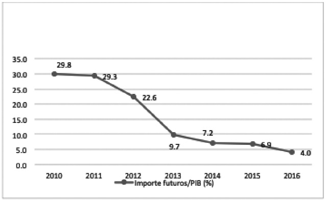
Source: elaborated with data from INEGI and MexDer.
Figure 1 Annual Amount of Futures Transactions in relation to GDP (%)
This speculative process of banking institutions and treasuries of large companies should not ignore that more unstable financial markets allow for the development of a variety of futures contracts. These derivatives manage to hedge the risk to institutions and investors (Mishkin, 2014), as the contract provides an underlying asset (Commodities, exchange rate, interest rate, etc.) that is standardized, set at a future date, and at a price agreed to in the present. This generated liquidity and financial engineering processes in favor of the companies3. And the markets turn out to be a viable modality when investments or the level of leverage are associated with risks and uncertainty, issues that traditional markets do not solve. In the period, futures transactions were generally made on 91-day CETES rates, stock index (IPC), 28-day TIIE, and Federal Government Development Bonds (M10 and M20). In 2016, the main contracts were for the 28-day TIIE and the IPC, in addition to contracts with various term bonds.
Methodology
The volatility analysis was carried out with monthly statistical series of futures contracts for the January 2010 to December 2016 period, with a total of 84 observations. The source of information was Mercado Mexicano de Derivados S.A. (MexDer) (Mexican Derivatives Exchange). It must be considered that the volatility in this work was applied taking the monthly amounts of the futures contracts, and then both the fluctuations of the Stock Exchange Index (IPC) and the interest rate of 28-day CETES were used as underlying assets.
The degree of volatility can be identified by applying processes such as GARCH (Generalized Autoregressive Conditional Heteroscedasticity), a first-order estimation model. In the GARCH process (1.1) it is observed that the volatility in time t depends on the volatility in the immediate past (t-1), thus it is deduced that these models are appropriate in the face of large fluctuations. Since the volatilities of a past period are included, they become useful in long periods of instability and calm (Aguirre et al., 2013). The advantage of this method is that it is not necessary to know the distribution function of a variable, in the case of an underlying asset, in order to achieve good instrumentation and measurement.
In the case of residuals, the GARCH model allows proving the existence of volatility, which makes its estimates more efficient than those obtained with the ARCH model. In Bollerslev (1986), a variance of estimates from previous periods was added to the equation in order to obtain a GARCH-type dynamic volatility (p, q) 4. In Bollerslev, Engle, and Nelson (1994), they state that the GARCH process is applied to a conditional volatility of two regression equations:
Where k is the variable or the yield of the underlying asset in time t, and Ɛ is the disturbance term, or white noise, whose residuals have zero mean and the variance is constant. In a long period of time, σ is the coefficient of volatility in time t, and Z is the random or stochastic variable with an ARMA (Autoregressive-moving-average model) structure, which is specified in the second equation (Arango and Arroyave, 2016; De Jesús, 2008; Aguirre et al., 2013).
To have a strictly positive volatility with the GARCH process, the estimated parameters need to comply with αo> 0, α1≥0, and β1≥0, as well as the sum α1 + β1 ≤1. The unconditional variance of error terms ε will be finite, with a strictly stationary and ergodic estimation of parameters5. It is necessary to verify that the series of the contract amounts, in the face of different assets, are shown correlated the error term ε and with the past in order to determine that it was stationary.
In some cases, ARCH (Autoregressive Conditional Heteroscedasticity) processes were applied to be able to compare with the estimated GARCH parameters. It happens with ARCH that although the moving averages of the square residuals are used, these are based on the yields from one or more periods that have many lags. The ARCH (p) process is consistent with the use of the following variance polynomial (Engle, 1982, 2001):
The parameters are αo>0 and the rest tend to be positive αi ≥ 0.
In general, the quasi-maximum likelihood method and Stata software were used for a better estimation of parameters with the ARCH and GARCH processes. This resulted in more robust standard errors, and in the assumption that the variations follow a normal distribution.
Valuation and volatility in futures contracts
The valuation of these contracts is largely dependent on the behavior of the underlying asset, mainly bonds and stock indices; every time the interest rate becomes a risk and has an erratic movement, it leads to a stochastic process (De Jesus & Diaz, 2011), consequently, investment preferences lean towards 3 and 10, or more, year bonds.
The significant flow of funds in futures contracts is explained not only by the volatility of the markets, but also by the need to ensure a level of liquidity in the future. Risks are raised by market swings in oil prices, stock market cracks, exchange rate devaluations, and interest rate adjustments (Gamboa and Vega, 1998). The creation and use of these instruments, accompanied by the use of various underlying assets, turn out to be an investment mechanism, while at the same time conserving value over time, liquidity, and fixing future prices, thus becoming a form of risk transfer (Chorafas, 1996; Gamboa and Vega, 1998).
The way trades move, and the prices that contracts have are crucial in the futures market.
This price can be expressed based on the following equation:
F: |
Futures price |
S: |
Price of the underlying asset |
Rt: |
Base risk (difference between the former price and the current price) |
C: |
Implicit transaction costs6 |
R0 : |
Zero-time risk assessment |
εt-1: |
Error term, delayed by one period |
In statistical work, the current futures and spot prices have small deviations. This is attributed to the good functioning of the arbitration mechanisms and, consequently, the negotiations become efficient and viable. When there is a difference between the futures price and the current spot value, the “base risk” (Rt) appears. This should be zero when approaching the delivery date, but this is not the case in the reality of how markets operate. Therefore, the lack of arbitrage opportunities leads to greater risk (Hull, 2017:75).
For Elvira and Larraga (2008), a valuation of the futures contract under the backing of a stock exchange index has another formulation. It is based on the conditions of a stock market, considering that this index presents adjustments in those shares, whose issuers have capital increases, but do not grant rights to dividends. The value of the futures contract must reflect the fluctuations of a portfolio of investment assets, the underlying value of which is the price index. Based on Hull (2009:108), the contract price is subject to the expression:
F: |
Futures value or price on a stock index |
St: |
Price of the underlying asset (Price Index) |
r: |
Risk-free interest rate in term |
d: | |
t: |
Delivery term |
Zt: |
Variables that are not implicit in the underlying asset (r, d, etc.) |
In this formulation, if F>St.Zt, it is advisable to invest in the futures contract, encouraged by probable profits; conversely, if F<StZt it is advisable not to invest because of expected losses. This could help in the representation of the ups and downs that occur in the markets, but it has limitations. Futures transactions and arbitration transactions, which actually occur in the markets and happen between buyers and sellers of contracts, are not contemplated.
Discussion of the results
The free flow of capital abroad creates the conditions to generate sufficient confidence and certainty regarding the stability of the exchange rate. Nevertheless, some authors establish that this marks the priority in the economic policy, that of avoiding speculation and of preventing “unhinging” the capital markets and currencies (Huerta, 2009). Stability in the markets should be supported by fiscal discipline and a controlled management of the exchange rate, despite the adjustments that took place at the end of 2016 and throughout 2017.
The efficient management of financial assets and liabilities is certainly subject to the ups and downs of the markets and the search for greater valuation of securities, accompanied by an updated flow of future returns. Nevertheless, it is possible that, given the volatility of the markets, it may be preferable to maximize returns or to fix the price of the foreign currency today until a certain future date (Kozikowski, 2000; Pacheco and Urzúa, 2003), based on the purchase of a derivative instrument, such as futures.
Structure and composition of futures transactions
Initially, futures investments were based on the interest rates of 91-day CETES and then they moved to equilibrium interbank interest rates. This shift in futures contracts was caused by falling oil prices and increasing exchange rate fluctuations. The predominance of uncertainty made investors prefer migrating to other types of contracts. According to MexDer data, there were futures transactions totaling 3.9 trillion current pesos in 2010, most of which were earmarked for equilibrium interbank interest rates (TIIE) and 91-day CETES. While in 2016 they totaled $756.9 billion pesos, and were earmarked to strong investments backed by the stock index (IPC), but not on interest rates (Table 1).
Table 1 Composition of futures contracts by type of underlying asset, 2010-2016 (Millions of current pesos)
| CONCEPT | 2010 | % of the Total |
2011 | % of the Total |
2012 | % of the Total |
2013 | % of the Total |
2014 | % of the Total |
2015 | % of the Total |
2016 | % of the Total |
| STOCK INDICES SUBTOTAL | 441,265.8 | 11.1 | 441,017.7 | 10.3 | 422,145.9 | 12.0 | 397,541.0 | 25.3 | 422,787.7 | 33.8 | 518,095.0 | 41.6 | 496,334.3 | 65.6 |
| IPC | 441,265.8 | 11.1 | 441,017.7 | 10.3 | 422,145.9 | 12.0 | 397,541.0 | 25.3 | 414,774.4 | 33.2 | 480,302.8 | 38.6 | 449,686.8 | 59.4 |
| Mini IPC | 8,013.2 | 0.6 | 37,792.2 | 3.0 | 46,647.6 | 6.2 | ||||||||
| RATES SUBTOTAL | 2,986,015.9 | 75.4 | 3,174,489.2 | 74.4 | 2,697,926.1 | 76.5 | 1,003,976.4 | 63.9 | 705,683.7 | 56.5 | 567,596.7 | 45.6 | 54,341.0 | 7.2 |
| CETES 91 | 375,856.9 | 9.5 | 327,827.1 | 7.7 | 167,880.2 | 4.8 | 46,140.9 | 2.9 | 4,660.0 | 0.4 | 0.0 | 0 | 0.0 | |
| TIIE 28 | 2,610,159.0 | 65.9 | 2,846,662.1 | 67.7 | 2,530,045.8 | 71.7 | 957,835.4 | 60.9 | 701,023.7 | 56.1 | 567,596.7 | 45.6 | 54,341.0 | 7.2 |
| BONDS SUBTOTAL | 534,059.6 | 13.5 | 653,941.6 | 15.3 | 406,605.4 | 11.5 | 169,828.1 | 10.8 | 120,807.9 | 9.7 | 158,700.4 | 12.8 | 206,284.2 | 27.3 |
| SHARES SUBTOTAL | 40.3 | 0.0 | 169.3 | 0.0 | 1.9 | 0.0 | 175.1 | 0.0 | 162.2 | 0.0 | 37.9 | 0.0 | 38.5 | 0.0 |
| SUM | 3,961,381.7 | 100.0 | 4,269,617.7 | 100.0 | 3,526,679.3 | 100.0 | 1,571,520.6 | 100.0 | 1,249,441.4 | 100.0 | 1,244,439.0 | 100.0 | 756,997.9 | 100.0 |
Source: elaborated based on the data from the Mexican Derivatives Exchange (MexDer).
This management and distribution of risks falls on the configuration of futures contracts, which, from 2010 to 2016, showed a dynamic in favor of underlying assets such as interest rates known as 28-day TIIE, which absorbed 65.9% in 2010 and fell to 7.2% in 2016, because the volatility of the exchange rate had a greater impact and there was no longer certainty in the direction of currency prices. On the other hand, futures based on stock indices (IPC) were the most promising and growing investment alternative, moving from 11.1% of the total in 2010 to 59.4% in 2016.
Concerning bonds as underlying assets, futures absorbed 13.5% of the total resources in 2010, and 27.3% in 2016 (Table 2). The most important instruments in these futures contracts were 3-year bonds (M3), 10-year bonds (M10), 20-year bonds (M20), and in 2016 the bonds maturing in December rebounded (DC24). When it came to shares and Certificados de Participación Ordinaria (CPO) (Ordinary Participation Certificates) included in the operations of the MexDer, the futures did not really show that there were strong investments in them. However, there were reports of movements and futures transactions of América Móvil, Cemex CPO, Grupo Mexico B, and Walmex V, among others.
Table 2 Futures contracts by type of bond and stock, 2010-2016 (Millions of current pesos)
| CONCEPT | 2010 | % of the Total |
2011 | % of the Total |
2012 | % of the Total |
2013 | % of the Total |
2014 | % of the Total |
2015 | % of the Total |
2016 | % of the Total |
| BONDS SUBTOTAL | 534,059.6 | 13.5 | 653,941.6 | 15.3 | 406,605.4 | 11.5 | 169,828.1 | 10.8 | 120,807.9 | 9.7 | 158,700.4 | 12.8 | 206,284.2 | 27.3 |
| DC18 | 3,681.5 | 0.3 | 38,100.8 | 5.0 | ||||||||||
| DC24 | 145,754.0 | 11.7 | 168,183.4 | 22.2 | ||||||||||
| 3-year bond (M3) | 116,421.3 | 2.9 | 21,333.5 | 0.5 | 29,423.5 | 0.8 | 32,492.5 | 2.1 | 28,749.6 | 2.3 | 2,497.2 | 0.2 | ||
| 10-year bond (M10) | 259,158.9 | 6.5 | 335,572.6 | 7.9 | 192,554.7 | 5.5 | 38,787.6 | 2.5 | 6,180.9 | 0.5 | 19.1 | 0.0 | 0.0 | |
| 20-year bond (M20) | 158,479.4 | 4.0 | 252,012.2 | 5.9 | 148,617.8 | 4.2 | 98,427.2 | 6.3 | 16,852.8 | 1.3 | 0.0 | 0.0 | ||
| 30-year bond (M30) | 45,023.3 | 1.1 | 36,009.4 | 1.0 | 120.9 | 0.0 | 2,263.0 | 0.2 | 1,865.3 | 0.1 | 0.0 | |||
| DC24 bond | 57,207.9 | 4.6 | ||||||||||||
| MY31 bond | 9,553.8 | 0.8 | 4,883.4 | 0.4 | ||||||||||
| SHARE SUBTOTAL | 40.3 | 0.0 | 169.3 | 0.0 | 1.9 | 0.0 | 175.1 | 0.0 | 162.2 | 0.0 | 37.9 | 0.0 | 38.5 | 0.0 |
| América móvil | 1.3 | 0.0 | 16.0 | 0.0 | 0.2 | 0.0 | 48.3 | 0.0 | 3.4 | 0.0 | 0.0 | |||
| Brtrac | 0.0 | 0.0 | 0.0 | 0.0 | 0.0 | 0.0 | 0.0 | 0.0 | 0.0 | |||||
| Cemex CPO | 0.0 | 0.0 | 15.2 | 0.0 | 1.7 | 0.0 | 0.0 | 2.7 | 0.0 | 2.3 | 0.0 | |||
| FemsaL Femsa UBD | 0.0 | 0.0 | 0.0 | 0.0 | 0.0 | 0.0 | 8.7 | 0.0 | ||||||
| Gcarso A1 | 0.0 | 0.0 | 0.0 | 0.0 | 12.7 | 0.0 | 0.0 | |||||||
| Gmexico B | 31.3 | 0.0 | 0.0 | 0.0 | 120.1 | 0.0 | 150.0 | 0.0 | 1.1 | 0.0 | 38.5 | 0.0 | ||
| Ilctrac | 1.7 | 0.0 | 0.0 | 0.0 | 0.0 | 0.0 | ||||||||
| Mextrac | 0.0 | 0.0 | 0.0 | 0.0 | 0.0 | 0.0 | 0.0 | |||||||
| Walmex V Walmart | 39.1 | 0.0 | 104.9 | 0.0 | 0.0 | 0.0 | 6.7 | 0.0 | 6.1 | 0.0 | 13.1 | 0.0 | 0.0 | |
| corn | 0.0 | 0.0 | 0.0 | 0.0 |
Source: elaborated based on data from the Mexican Derivatives Exchange (MexDer).
GARCH process and general results analysis
In the futures market, the analysis of the series of monthly contract amounts in the 2010 to 2016 period shows an average of 26,403.3 million current pesos per month (Table 3). There is enormous variability in contract amounts; from a minimum of 5,108.6 to a maximum of 122,935.6 million pesos per month. The asymmetry was of 3.0 and a coefficient of kurtosis of 12.7, the distribution of which managed to possess a high concentration around the mean and a great peak towards the side (leptokurtic) (Figure 2).
Table 3 Basic Indicators, 2010-2016
| Descriptive Statistic | |
| Mean: | 26,403.3 |
| Standard Deviation: | 17,698.1 |
| Asymmetry: | 3.0 |
| Kurtosis: | 12.7 |
| Median: | 22,959.8 |
| Minimum: | 5,108.6 |
| Maximum: | 122,935.6 |
| Q 1: | 17,004.6 |
| Q 3: | 31,510.7 |
Source: elaborated with data from the MexDer
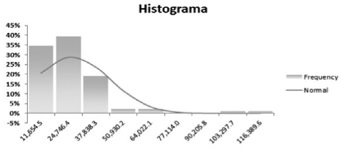
Source: own elaboration with data from the MexDer.
Figure 2 Distribution of data throughout the 2010-2016 period
Taking the monthly amounts of the futures contracts, which comprises 84 observations, the linear GARCH method was applied between 2010 and 2016, resulting in positive conditional volatility, and the conditional variance was not constant. Three rules are met:
The parameter estimation is positive (αo=996.3 million, α1=0.01, and β1=0.01) for the three cases of GARCH (1,1): normal distribution, t-student, and generalized error distribution (GED) (Table 4).
These estimated parameters (α1 + β1) <1 imply that there is persistence in terms of the speed of error reversal concerning the mean. The GARCH process (1,1) is strictly stationary and ergodic, as the conditions of being convergent and congruent with a greater approach to the mean are met as the size of the sample grows.
In particular, parameter β1 is different from 0, although it is close to zero. This indicates that the distribution of the amount series of the monthly contracts does not have a thick tail towards one of the sides.
Table 4 GARCH application in futures: estimated parameters
| Parameters | GARCH-values (1,1) [Normal Distribution] | GARCH-values (1,1) [T-Student] | GARCH-values (1,1) [Generalized Error Distribution (GED)] |
| µ | 26,403.31 | 26,403.31 | 26,403.31 |
| a0 | 996,318,857.56 | 996,318,857.56 | 996,318,857.56 |
| a1 | 0.01 | 0.01 | 0.01 |
| b1 | 0.01 | 0.01 | 0.01 |
| v | - | 5.00 | 2.00 |
| Tests | p-Value | Significance | |
| White noise | 37.41% | True | |
| Normal Distribution? | 0.00% | False | |
| ARCH effect? | 99.28% | False | |
| Residual Objective | P-Value | Significance | Significance test at 5.00% |
| 0 | 0.00% | True | |
| 0 | 0.00% | True | |
| 0 | 0.00% | True |
Source: elaborated based on data from the MexDer.
The non-negativity of parameters α and β, as well as the other rules, means that there is no impediment in accepting the estimates through the GARCH process. The hope of the GARCH model (p, q) is zero, and the variance will be distributed in a homoscedastic manner throughout the period.
Based on these parameters, the GARCH models produce estimates within the sample for the daily yields of futures prices for the period, using the quasi-maximum likelihood method, which provides more robust standard errors, assuming that the variations follow a normal distribution. From the results of the near-maximum likelihood parameters of the GARCH model, it is possible to see that all the estimators are statistically significant at the different levels of significance.
Similarly, for the parameters of the conditional variance equation, the GARCH model (1,1) of these futures contracts does not show dynamic patterns of conditional volatility, such as financial belief. The estimated parameters are statistically significant in the most common confidence intervals.
In this analysis the evaluation of the null hypothesis is carried out. Considering the p-value, the white noise test provides a determining result on the yields generated by the movements in the amounts of the futures contracts. The low significance of the GARCH model clearly shows that there is no serial autocorrelation in the futures price yields, and thus accepts the null hypothesis of white noise process in the series, particularly in the yields for any level of significance.
Conversely, the parameters obtained with the application of the normal distribution and the ARCH effect provide unsatisfactory results. When analyzing the residuals, the error term (εt) follows a conditional normal distribution, with zero mean and constant variance (σ2), which allows inferring that the estimates are significant. Consequently, the results show strong evidence of a high degree of persistence in the process of conditional volatility in futures prices.
Volatility when the underlying asset is the stock market index (IPC)
The analysis of conditional volatility and the stochastic processes deserve scrupulous attention when the underlying asset is the Stock Exchange Prices and Quotations Index (IPC). The yields and volatility of this index are representing investment opportunities, valued in futures contracts. In essence, futures trading depends more on how the prices of the underlying assets move (Zhong, Darrat, and Otero, 2004). This is the case with the stock index, which reflects all the movements of the shares7. As a result, futures valuations no longer have an exclusive underlying asset in reference to spot commodity prices, under the belief of ensuring a future price of these products.
The relation of the conditional volatility and the stochastic processes of the amounts in futures with the movements of the stock market index is observed. The monthly series of the IPC are taken, with 84 observations, which are analyzed with the GARCH process for the 2010-2016 period. This results in a mean of 40,521.7 points (Table 5). There is a marked variability in the behavior of the IPC, ranging from a minimum of 31,333 to a maximum of 48,011 points. The value of the asymmetry is -0.46, with a kurtosis of 2.13 (leptokurtic), reflecting a distribution with pointing.
Table 5 Descriptive statistic: stock index (IPC)
| Mean | 40,521.7 |
| Standard deviation | 4,507.3 |
| Variance | 20,300,000.0 |
| Variation coefficient | 0.11 |
| Asymmetry | -0.46 |
| Kurtosis | 2.13 |
| Range | 16,677.9 |
| Minimum | 31,333.6 |
| Maximum | 48,011.5 |
| No. of observations | 84 |
Source: elaborated with data from the MexDer.
The use of the ARCH process on the monthly amounts of these contracts leads to the estimation of positive parameters, such as: αo=1.10, α1=0.18, and β1=6.03. This reflects that the conditional volatility is positive, and that the conditional variance is not constant; this means that there is heteroscedasticity8 in consideration of lagging periods (t-1), and that the estimates may not be significant.
As for the application of GARCH (1,1) for the monthly series of amounts of the 20102016 futures contracts, a non-positive conditional volatility and the non-consistent conditional variance are described. This is based on three rules:
The estimation of parameters is not all positive: αo=0.00, α11=0.02, and β1=-0.26, if a normal distribution of errors is considered. (Table 6).
These estimated parameters do not comply with: (α1 + β1) <1. This implies that the GARCH process (1,1) is not strictly stationary for the analyzed period.
The β1 parameter is different from 0 and has a negative value. This reflects that the distribution of the series of monthly amounts presents thick tails, but with tendencies towards values lower than the average and the median.
Table 6 ARCH and GARCH methods at stock market indices (IPC): estimated parameters
| Parameters | ARCH Values (1,1) | GARCH Values (1,1) |
| µ | 40,759.87 | 40,759.87 |
| α0 | 1.10 | 0.00 |
| α1 | 0.18 | 0.02 |
| β1 | 6.03 | -0.26 |
| v | 0.00 | 0.79 |
Source: elaborated with data from the MexDer.
In this occasion, the non-negativity of the estimated parameters is not met, because β<0 leads to not accepting the ARCH or GARCH estimates when the underlying asset incorporates the stock market index. Therefore, there is a heteroscedastic distribution of errors throughout the period.
The GARCH process, when the underlying asset is the IPC of the Stock Market, and considering the lagged terms of errors and variances, becomes a useful method based on the following observations:
It is able to predict the conditional variance and, therefore, volatility (Engel, 2001).
As a precondition, it is necessary to be sure that there is heteroscedasticity.
If the volatility is perceived to be high and persistent, then it becomes more dangerous.
This method is a tool that can provide reliable indications in the exposure to risk behavior of a stock market.
In this case, the 2010-2016 period implies the use of more than 2000 daily observations, which shows the unstable and volatile behavior by sections. The most significant changes in price variability occurred between 2014 and 2015-surmised in the sequence from 1450 to 1600 observations in Figure 3-due to strong fluctuations in the stock market index, in the face of sharp falls in oil prices and the influence of other variables. To identify the non-consistency of the variance and the growth of the volatility, the ARCH model was used first, followed by the GARCH model, which was the most useful in estimating the variances by means of a weighted average of the square of the residuals and the series of past lags.

Source: elaborated with data from the MexDer.
Figure 3 Evolution of daily yields of futures contracts based on the Stock Exchange Prices and Quotations Index
Figure 3 shows the series of daily volatilities, which reflect financial yields and have more or less stable periods of minimal differences in the variability of the price index (IPC). These volatilities are interspersed with high variability and instability from pronounced fluctuations, and then return to smaller and symmetrical fluctuations around the mean. It is possible to distinguish a grouping of volatility, with relative persistence and reversion to the mean. Conditional homoscedasticity is evident in certain sections, which then returns to conditional dispersion or heteroscedasticity, which is known as clustering or volatility in agglomerations (Engle, 1982; Bollerslev, 1986).
In addition to this situation, there are changes in the variance from one period to another, which do not occur randomly. There are periods of low volatility and equal variance, followed by periods of rising volatility, then declining again and being stable. All this implies that the variance of errors and volatility are unavoidably associated for the case of futures and the Stock Exchange Prices and Quotations Index.
Volatility of futures with respect to interest rates
Based on the 28-day CETES interest rates of the Bank of Mexico as the underlying futures value, the stochastic process of these monthly average rates became determinative in the amounts of the futures contracts. A low volatility of interest rates was observed, with a variation coefficient of 16.7% with respect to the average. This average ranged between 2.67% and 5.61% in the period, its maximum value. The mean was of 3.82%. The variance of the sample was 0.41 and had a kurtosis of -0.70, which reflects a less targeted distribution (platykurtic) with thicker tails (Table 7).
Table 7 Descriptive Statistics: 28-Day Cetes Rates
| Mean | 3.82 |
| Typical error | 0.07 |
| Median | 4.04 |
| Mode | 3.02 |
| Standard deviation | 0.64 |
| Variance of the sample | 0.41 |
| Variation coefficient | 0.16 |
| Kurtosis | -0.70 |
| Asymmetry Coefficient | -0.10 |
| Range | 2.94 |
| Minimum | 2.67 |
| Maximum | 5.61 |
| No. of Observation | 84 |
Source: elaborated with data from the MexDer
The GARCH method applied to the monthly series of interest rates from 2010 to 2016, to estimate the behavior of conditional variance, square residuals, and conditional volatility, will be strictly positive and adhere to the GARCH process (1,1). For this, at least two rules must be followed:
The parameters αo=0, α1=0.51, and β1=0.51 are positive in the three GARCH situations (1,1): normal distribution, t-student, and generalized error distribution (GED) (Table 8).
As the estimated parameters (α1 + β1)>1, the unit is slightly exceeded, which means that the GARCH process (1,1) gives a slight non-persistent variance. There is no strictly stationary process for the determination of the conditional variance.
Table 8 GARCH method at CETES interest rates: estimated parameters
| Parameters | GARCH-Values (1,1) [Normal Distribution] | GARCH-Values (1,1) [T-Student] | GARCH-Values (1,1) [Generalized Error Distribution (GED)] |
| µ | 3.82 | 3.82 | 3.82 |
| a0 | 0.00 | 0.00 | 0.00 |
| a1 | 0.51 | 0.51 | 0.51 |
| b1 | 0.51 | 0.51 | 0.51 |
| v | - | 5.00 | 2.00 |
| Tests | p-value | Significance | |
| White Noise | 0.00% | False | |
| Normal Distribution? | 37.22% | True | |
| ARCH effect? | 0.00% | True | |
| Residual Objective | P-Value | Significance | Significance Test at 5.00% |
| 0 | 0.00% | True | |
| 0 | 36.21% | False | |
| 0 | 7.21% | False |
Source: elaborated based on data from Bank of Mexico.
With the compliance of these rules, given the non-negative parameters α and β, it is possible to accept the GARCH estimates with respect to the three conditions: normal distribution, t-student, and generalized error distribution.
There is a kurtosis of -0.70 and a parameter of β1=0.51, which is b1 different from 0. It is evident that the queues of the distribution of the interest rates are thicker than normal in light of the description of an almost flat kurtosis, without peak.
An evaluation of these parameters, if the existence of white noise is considered, shows futures not achieving decisive results on yields and volatility, taking into consideration interest rates. On the other hand, the parameters resulting from the normal distribution and the application of the ARCH Effect, which contemplates the most recent past to estimate the variance of a period, do present determining results on the yields of interest rates. The significance test at 5% of the squared residuals, for the error term (εt) follows a conditional normal distribution, with zero mean and a constant variance (σ2); this warns of a strong confidence and precision in the estimated parameters.
Conclusions
The use of the GARCH method and, in certain cases the ARCH method, provides a satisfactory estimate of the degree of conditional expected volatility in relation to various underlying assets in futures contracts. The estimated parameters show that the GARCH process is more acceptable, even if the errors are not distributed normally. It should be noted that the volatility measurement involved the monthly amounts of the contracts. However, the results move significantly when the statistical series changes and the Stock Exchange Index and the CETES interest rates are used.
With persistent volatility in the price index and bond yields, investors have an unpredictable behavior as to whether this will help them make decisions regarding futures contracts. Investors expect a higher return when there is a higher, risk-adjusted profitability (Crane et al., 1995). As has already been shown, futures contracts depend on how volatile the stock market is in order for the price index of this instrument to be taken as a reference for the underlying asset.
Despite criticism and comments, the GARCH model is useful and is a key tool in analyzing the behavior of risk exposure in futures markets in particular. Perhaps in other financial markets it is not as useful, due to the degree of volatility and because it is more persistent and dangerous. In emerging economies, it is attributed to a strong weakness in their institutional and financial structures.
Futures transactions reflect investment opportunities, depending on whether the futures price is a good investment alternative. These contracts had an upward behavior in terms of amounts of investments and as a result of the fact that the decisions are supported with the certainty in the future price. Indeed, this should not represent a loss in the negotiation of a futures contract. In addition, futures investments may yield possible expected profits, as contracts include one or more underlying assets, whose interest rate generates encouraging expectations in the long term.
REFERENCES
Abascal, Mario (2016). Análisis de series temporales financieras. Trabajo de fin de grado, Grado en Economía 2015-2016, Universidad de Cantabria, 30 de junio 2016, pp. 1-29. [ Links ]
Aguirre, Alejandro; Vaquera, Humberto, Ramírez, Martha, José R. Valdez & Carlos A. Aguirre (2013). “Estimación del valor en riesgo en la BMV usando modelos de heterocedasticidad condicional y teoría de valores extremos”. Economía mexicana, nueva época, vol. XXII, No. 1, revista del CIDE, primer semestre 2013, pp. 177-205. [ Links ]
Ang, J. B. (2010). “Does foreign aid promote growth? Exploring the role of financial liberalization”. Review of Development Economics, 14(2), pp. 197-212. [ Links ]
Arango, Mónica & Arroyave, Santiago (2016). “Análisis de combustibles fósiles en el mercado de generación de energía eléctrica en Colombia: un contraste entre modelos de volatilidad”. Revista Métodos Cuantitativos para la Economía y la Empresa, No. 22. Sevilla, España: Universidad Pablo de Olavide, diciembre, 2016, pp. 190-215. [ Links ]
Bariviera, Aurelio; Basgall, Maria J.; Hasperue, Waldo y Marcelo Naiouf (2017). Some stylized facts of the Bitcoin market. Physica A: Statistical. Published by Elsevier. August 16, 2017. [ Links ]
Bollerslev, T., R. F. Engle & D. B. Nelson. (1994). ARCH models. In R. F. Engle and D. L. McFadden (Eds.), Handbook of Econometrics IV, Amsterdam: Elsevier Science, 2961-3038. [ Links ]
Bollerslev, T. (1986). “Generalized Autoregressive Conditional Heteroskedasticity”. Journal of Econometrics, 31, 307-327. [ Links ]
Chesnais, Francois (2000).”¿Crisis financieras o indicios de crisis económicas características del régimen de acumulación actual?”. En Chesnais, F. & D. Plihon (Coordinadores). Las Trampas de las Finanzas Mundiales. Madrid: Akal. [ Links ]
Chorafas, Dimitris (1996). Practical Introductions to Advanced Financial Analysis: Markets and the Instruments which they Fund. London: Euromoney Publications. [ Links ]
Coase, Ronald (1937). “The Nature of Firm: Origin”. Economica, New Series, Vol.4, Issue 16 (Nov., 1937), pp. 386-405. [ Links ]
Crane, D.B. Froot, K. A., Mason, S. P.; Perold, A.; Merton, R. C.; Bodie, Z. & Tufano, P. (1995). The Global Financial System: a Funcional Perspective. [ Links ]
De Jesús, Raúl (2008). Riesgo y volatilidad en los mercados accionarios emergentes: Medición del VAR y CVAR aplicando la teoría de valor extremo. Tesis de Doctorado en Ingeniería. México: Facultad de Ingeniería, UNAM. [ Links ]
De Jesús, Raúl & Miguel A. Díaz (2011). “Soluciones de forma cerrada para la valuación de opciones con tasa de interés estocástica bajo una medida forward neutral al riesgo”. Estocástica, finanzas y riesgo, No.2, Año 1, julio-diciembre 2011, UAM-A, Depto. de Administración, pp. 7-33. [ Links ]
Dyhrberg, Anne H. (2015). “Bitcoin, gold and the dollar: A GARCH volatility analysis”, Working Paper Series, UCD Centre for Economic Research, No.15/20. [ Links ]
Elvira, Oscar & Pablo Larraga (2008). Mercado de Productos Derivados. Barcelona: Bresca Editorial. [ Links ]
Engle, Robert (2001). The Use of GARCH/ARCH Models in Applied Econometrics. Journal of Economic Perspectives, 4, 157-168. [ Links ]
Engle, Robert (1982). “Autoregressive Conditional Heterocedasticity with Estimates of the Variance of United Kingdom Inflation”. Econometrica, No.4, Vol. 50, (july), pp. 987-1008. [ Links ]
Gamboa, Gerardo & Francisco Vega (1998). “Ventajas de la incorporación de productos derivados en las sociedades de inversión”. Sociedades de Inversión, No.2. México: Grupo de Asesores Financieros (GAF)-Ediciones y Gráficos Eón S.A. [ Links ]
Girón, Alicia (2010). “Acciones especulativas y desplomes financieros”. Economía Informa, No. 362. México: UNAM-FE, enero-febrero 2010, pp. 17- 22. [ Links ]
Grimmett, G.R. & D.R. Stirzaker (1992). Probability and Random Process. 2a. edición. New York: Oxford University Press. [ Links ]
González, G.; Mora, A. y G. Solano (2015). “Empleando diferentes métodos de estimación de la volatilidad”. Estudios Gerenciales, 31 (136), pp. 287-298. http://doi.org/10.1016/j.estger.2015.03.004 [ Links ]
Huerta, Arturo (2009). “La autonomía del Banco Central y su inoperatividad a favor de la dinámica económica”. En Flores, Daniel; Ma. Lourdes Treviño y Jorge Valero (Coordinadores). La economía mexicana en 19 miradas. México: UANL-M.A. Porrúa. [ Links ]
Hull, John C. (2017). Options, Futures and Other Derivatives. 10th edition. USA: Pearson. [ Links ]
Hull, John (2009). Introducción a los mercados de futuros y opciones. 6a. edición. México: Pearson Educación de México S.A. [ Links ]
Katsiampa, Paraskevi (2017). Volatility estimation for Bitcoin: Acomparison of GARCH models. Economics Letters 158 (3),(6). Published by Elsevier B.V. [ Links ]
Kozikowski, Zbigniew (2000). Finanzas Internacionales. México: McGraw-Hill. [ Links ]
Mettenheim, Kurt (2013). Back to basics in banking theory and varieties of finance capitalism. Accounting, Economics and Law, 3(3), 357-405. [ Links ]
Miller, Merton H. (1992). Financial innovations and market volatility. New York: The Free Press. [ Links ]
Mishkin, Frederic (2014). Moneda, banca y mercados financieros. Edit. Pearson, 10ª. Edición. [ Links ]
Ontiveros, Emilio (1994). “Merton H. Miller: Financial innovations and market volatility”. Revista de Economía Aplicada, No.4 (Vol. 11), pp. 205-210. [ Links ]
Orhangazi, O. (2015). “Financial deregulation and the 2007-08 US financial crisis”. In Hein, E., Detzer, D., Dodig, N. (eds.), The Demise of Finance-dominated Capitalism: Explaining the Financial and Economic Crises. Cheltenham: Edward Elgar. [ Links ]
Pacheco, Cristina & José de J. Urzúa (2003). “Instrumentos financieros del mercado de derivados que se manejan en México”. Mercados y Negocios, Vol. 8, año 4, julio-diciembre 2003, pp. 41-48. [ Links ]
Soto, Roberto (2010). “Desregulación financiera y finanzas en México”, Economía Informa , No. 362, México: UNAM-FE , enero-febrero 2010, pp.48-58. [ Links ]
Tsay, R.S. (2002). Analysis of financial time series. Nueva York: John Wiley and Sons, Inc., 448 pp. [ Links ]
Vershik, Ana (2000). Derivados Financieros y de Productos. Buenos Aires: Ediciones Macchi. [ Links ]
Zhong, Maosen; Ali Darrat & Rafael Otero (2004). “Price discovery and volatility spillovers ind index futures markets: Some evidence from Mexico”. Journal of Banking and Finance, 28 (12), pp. 3037-3054. [ Links ]
1For John Hull (2009, 2017), these are underlying asset-backed securities. A yield or premium is earned, deriving from the original price or purchase price.
2Volatility is identified by the conditional variance of returns on certain assets, such as the underlying assets in futures contracts (Tsay, 2002; Aguirre et al., 2013).
3It is the use of financial engineering to “translate” gains and losses over a time horizon from derivatives, from hypothetical to future value. This made it possible to “manipulate financial statements and pay less taxes” (Soto, 2010: 54-55).
4The GARCH model (p,q) considers p to be the number of terms lagging from the squared error and q to be the terms of the lagged conditional variances. The GARCH model (1.1) has proven to be extremely useful for predicting conditional variance, and hence volatility (Engel, 2001).
5These conditions are fulfilled under the ergodic theorem, an independent distribution of the mean where the mean has convergence towards that point, in light of larger samples (Grimmet & Stirzaker, 1992).
6For Ronald Coase (1937), transaction costs have to be considered in exchanges, because they represent an externality, but this externality opens the possibility of an innovation process and market efficiency.
7There are works (Zhong, Darrat, and Otero, 2004) that show that the futures market uses the stock market index as an underlying asset, and it is a faithful reflection of stock prices; however, its volatility becomes a source of instability.
8If the variance of errors is not constant it is known as Heteroscedasticity, and may give incorrect estimates of the coefficients (Engel, 2001).
Received: October 24, 2017; Accepted: June 28, 2018; Published: October 29, 2019
 Este es un artículo publicado en acceso abierto bajo una licencia Creative Commons
