


 nova página do texto(beta)
 Inglês (pdf)
 Artigo em XML
 Referências do artigo
 Enviar este artigo por email
 Citado por SciELO
  Similares em
SciELO
Similares em
SciELO 
 Permalink
Introduction
Climate change related risks are increasing rapidly with highly vulnerable communities living in different conditions: cities, countryside and informal settlements. The likely direct impacts of climate change and climate variability include extreme precipitation, heat stress, pluvial and fluvial flooding, landslides, drought, increased aridity, and water scarcity with widespread indirect impacts on people, economies and ecosystems (Revi et al, 2014).
Climate change is expected to have severe effects on the populations of developing countries because many of them depend heavily on agriculture for income, have large impoverished rural populations which rely on agriculture for subsistence, and are financially and technically least equipped to adapt to changing conditions (Seaman et al, 2014). Therefore, planning measures to support adaptation to reduce the impact of climate change on poverty and food security requires methods of identifying vulnerable regions at national and local levels.
The Intergovernmental Panel on Climate Change (IPCC) expects that climate change will have major impacts in the near-term based on extreme precipitation and drought in developing countries. This will lead to shifts in the production areas of food and non-food crops and will have major impacts on food security and agricultural incomes, with a disproportionate impact on the welfare of the rural poor (IPCC, 2015).
However, adaptation and mitigation policies remain scarce in middle-income countries. Finite resources and technological capacity restrict the ability of adaptation strategies in social systems, primarily in developing countries (Kates et al, 2012; Moser and Ekstrom, 2010).
In the particular case of Argentina, since 1960 there was a remarkable increase in precipitation over most of the subtropical region of the country. This has favored the increase in crops´ yields and also the expansion of crop lands into semiarid regions (Barros, 2015). This effect, among other economic factors such as the Asian miracle and increase in technology (Massot, 2016), made agricultural exports reach a share of 55% of total exports for the period 2003-2016. Soybean, soybean oil and soybean meal contributed with 23% to the total valued exported in that period.
Despite research has been done in estimating crop´s reaction to different scenarios of increase of CO2 emissions, there is no research that take into account climate variability in the short term at a nationwide scale. The valuation of current and medium-term losses is a must to communicate the need of an adaptation strategy for the most vulnerable countries like Argentina.
Therefore, the objective of this study is to provide an estimate of income losses in soybean production in Argentina due to climate variability. These valuations may provide important information to plan adaptation strategies for a current problem, which should be taken by developing countries highly reliant on agricultural exports like the case studied. The objective of the study is to provide a general estimation of the magnitude of the economic loss to determine if the level of impact is local, regional or macroeconomic; and therefore discuss which kind of adaptation measures should be proposed.
The first section of this work summarizes different approaches to estimate crops reaction to weather events. The second section presents the selected model and data. Section three synthesizes results and section four and five presents further discussion and some concluding remarks.
Theoretical framework
When addressing the problem of impact valuation of climate change or climate risk, several problems arise: scale, kind of impact to measure, valuation methodology, prices projection and information availability.
Regarding the scale, valuation results will be totally different if the problem is analyzed globally, nationwide, or at a regional/local level. Studies at a global scale, they analyze impacts of a certain trend -global warming- or shock -drought or excessive rainfall-across countries and in the global economy. For instance, Burke et al (2015) conclude that unmitigated warming is expected to reshape the global economy by reducing average global incomes roughly 23% by 2100 and widening global income inequality due to different impacts between agricultural and industrialized countries with non-linear effect of temperature on economic production, relative to scenarios without climate change. As for shocks at a global scale, Cashin, Mohaddes and Raissi (2014) analyze the international macroeconomic transmission of El Niño weather shocks, concluding that the economic consequences differ across countries, considering variables such as economic activity or inflation.
Regarding nationwide approach (Aaheim, 2012; CIER, 2007; CEPAL, 2010; DNP BID, 2014; CEPAL, 2014), most value the impact over economic sectors (agriculture, fishery, forestry, transport, energy and water resources) and then summarized them into GDP estimates, in some cases through a general equilibrium macroeconomic model. However, this approach is related to CO2 emissions scenario and do not take into account climate variability.1 Also, linkages between sectors -such as the relation between water resources, energy and agriculture- are not monetary valued. Finally, as impacts of climate change are experienced locally (Carter et al, 2014), local scale approach has been more deeply studied by selecting a specific area of agricultural production or a field.
Therefore, selecting the scale will somehow define the scope of the problem to be analyzed, such as food security, rising prices or production loss. Regarding economic impact, it might be focalized in income or profit, or in the effect on prices. Therefore, valuation methodology will depend on scale and type of impact and can range from simple approaches (macroeconomic sensitivity) to more sophisticated cross sectional statistical methods or time series analysis (sensibility models, Ricardian models, loss function models, etc.).
However, sensibility estimation models require a large amount of information, and climate information availability is scarce in underdeveloped countries. Nevertheless, according to the data-base study performed by Gall (2015), loss estimates provide crucial, although incomplete, data for estudying the relationship between climate change and its effects on climate-sensitive hazards as well as loss and damage.
Lastly, when facing economic valuation, prices are not only a key element to be taken into account but also one of the most difficult variables to forecast. This is because all effects (economic, political, social, climatic and expectations) are somehow expressed on current prices. Isolating global commodities prices fluctuations due to specific climate events require a deep econometric analysis. Different approaches to evaluate impact on commodity prices can be consulted in Cashin et al (2014), Arteaga et al (2013) and Thomasz et al (2016).
This research studies the economic impact on the agricultural sector. Therefore, some of the most common and widely used approaches in agriculture such as, the agronomic, Ricardian and yields variability approaches are summarized below.
Agronomic approach
The agronomic approach estimates changes in yields due to technology, soil quality and of course climate events, among many other relevant variables. It is widely used in several studies, such as Lobell and Burke (2010), Rahman (2005), Paltasingh et al (2012), Chimeli et al (2008). The approach estimates sensibility coefficients through different methods -mainly least squares- in cross section data for different areas, or in a time series within one specific area. A general equation for this approach is:
Where,
Qrt: crop yield in a predefined county or region and for a certain time period (Paltasingh et al, 2012; Loyola et al, 2010; Lobell, 2010; Tannura et al, 2008). Ordaz et al (2010) estimates this production function using as dependent variable aggregate production indexes instead of a specific crop.
Art: area harvest for crop in county or region; VTrt: technological variables such as soil quality, seed genetics, and producer-level management techniques; VCrt climatic variables such as average and maximum temperature, accumulated rainfall; VS socioeconomic variables such as total population, total economically active population, and rural economically active population.
Different studies use a different set of variables to isolate the impact of climate variables over crop´s yields. For instance, Ordaz et al (2010) use socioeconomic data as a control variable because in their study agricultural production is labor intensive. On the other hand, impact of technology was incorporated by Tannura et al (2008) in a study of soybean and corn yields in Illinois, Indiana and Iowa.
This approach can be accurate to estimate the sensitivity of yields to climate variables. However, it does not provide economic estimations of losses produced by weather events and does not incorporate climate variability: changes through the years of the estimated coefficient are usually associated to climate change. Finally, it requires an extensive data set at local scales.
The hedonic approach
The hedonic approach, also called Ricardian method, is a popular method to estimate the effects of climate change over land value. It can be used to estimate the effects on the rent of land and also over agricultures benefits, according to different variations of the model.
In a perfect competitive market, land value equals present value of future profits generated by land’s production. Land income can be represented as follows:
Where pi is the crop`s price, Qi the production level, x represents input and wx is price of input x. Production level depends on technological (t), socioeconomic (s) and climatic variables (c). Producers choose x in order to maximize net income. Maximum net income is given by:
With the result of equation 3, land value is calculated as the present value of future income:
Where LVt is land value, and VTrt, VCrt and VSrt are vectors of technologycal, climatic and socioeconomical variables β0 is the intercept, βi,j the parameters coefficients and µt the stochastic error.
Deschenes et al (2007) employed the Ricardian approach to study the economic impact of climate change over the main crops produced by the USA. They modified the model to have profits instead land value as dependent variable:
Where are the profits of a region for year t, is a vector of climatic variables2 for the region for year t, is a vector of relevant variables in the determination of land value3. Factor represents the fixed effects for a region that absorbs every specific effect not observed by the dependent variable, is the intercept, the parameters coefficients and µt the stochastic error.
Yield variability approach
Another approach is the study of yields variability for a specific crop through a time series. Yields are affected by a complex combination of factors, such as weather, soil quality, seed genetics, and producer-level management techniques. However, despite this complexity, yields tend to show a general increase over time, which is commonly referred as the trend yield (Tanura et al, 2008).
The methodology estimates the yields` trend and study the deviation from it. Over empirical bases, it is then studied if those deviations can be explained by climate events.
There are many models to estimate the trend, such as linear and non-linear regression, polynomial adjustment, moving averages and local regression models. However, when studying crop yields` trends, the estimation of the trend is mainly done by a linear or log-linear model (Tanura and Irwin, 2015; Heinzenknecht, 2011; Beathgen, 2008; Thomasz et al, 2015). The equations of such models are:
Linear model:
Log-linear model:
Where yt is the actual yield in year t, xt is the time period, b0 is the intercept, b1 is the trend coefficient, and μt is the stochastic error. The absolute deviation from the trend is:
Where yt is the actual yield in year t, and
Where Rdt is the relative deviation,
dt is the absolute deviation and
Where k is the number of standard deviations that represent the limit from which yields are considered non-extreme from extreme. The selection of k is empirical and depends on the distribution of the sample.
Either classification allows identifying cases of yields` deviations that could potentially be explained by climate events. Having the potential cases, the following step it to analyze climate variables and determine if there was a climate shock in those years. Therefore, the approach identifies deviations that must be contrasted with a climate variable.
The methodology allows to easily identify extreme deviations of trended yields that are potentially explained by climate shocks. It is a simple approach which deals properly with scarce information. The trend estimation allows reconstructing a theoretical production for every year, in absence of climate variability. This means that the approach constructs a baseline or counterfactual scenario from which is possible to measure the production loss and consequently loss of income using different forecasts of prices.
Approach, methodology and data
Approach
The problem to be addressed in this work is the absence of a reliable and standardized model that can summarize a monetized income loss estimate in agricultural production due to climate events at a national/regional scale. The objective will be to provide estimates of income losses to determine the kind and scale of adaptation strategies. Therefore, this research starts with the valuation of past events, which could be taken into account to forecast into a mid-term future scenario.
The case to be studied is soybean production in the core area of Argentina, which represents 81% of national crop production and 77% of implanted area in 2016. It also represents an average of 23% of total value or exports between 2003-2016.
Methodology
To estimate income loss in soybean production the deviation from a linear trend model is used. The trend is adjusted through a linear model for two reasons. First, according to Irwin and Good (2015) log-linear model implies that the range of trend yield deviations in bushels should expand across time which clearly does not happen. It should also be noted that an important property of the linear trend model is that the percentage change in trend yields declines over time as the same bushel increase in trend yield is divided by a larger base. This is consistent with historical average soybean yields (Irwin and Good, 2015). Second, over empirical bases, in Thomasz et al (2015) was tested that the lineal model identifies all cases of draughts, while the log-linear model omits two cases.
Standard deviation of de-trended yields4 is calculated to identify extreme deviations. Extreme deviations are defined as those which exceed the limit of one standard deviation. 5 The aim of the study is to value production losses; therefore, only negative cases are analyzed.
The following step is to relate the extreme deviations in yields with climate events. In this work, the Palmer drought index will be used. Years of extreme deviations are compared to the index in the critical season of the crop. If drought levels are high, it is considered that the extreme deviation in yields were produced due to water shortage. Cases of extreme negative deviations which are not related to water shortage are not considered. In sum, any potential case has reach two attributes: be an extreme negative deviation from the yield`s trend and there has to be a drought in the area measured by the Palmer Index. Thresholds of both attributes will be further detailed and discussed.
It must be pointed out that there might be cases of low yields not captured by the model because they do not cross the threshold. However, as it was mentioned, the methodology focus only in extreme events, therefore is expected to have very little omitted cases.
When a case is identified, the production loss is estimated. To do this, the baseline scenario will be the yield trend plus one standard deviation, considering that within that interval fluctuations can be considered as non-extreme event. The quantity loss is multiplied by the price estimate to value the loss of income. Regarding price estimate, international soybean price will be used. We assume for our valuation that international prices are not affected by Argentinian soybean production, which are mainly driven by United States physical stocks. In this case, an average price of the year will be used.
The estimation methodology is presented below:
A liner trend is estimated from observed yields, from where estimated yield is calculated for every year of the sample:
Where,
The difference between the observed and estimated yield trend is calculated:
This de-trended series represents potential effects of climate variability over trends. To set a limit to define normal from extreme yields, the standard deviation is calculated,
Cases of
Estimation of yield loss is calculated as the difference of between
The theoretical level of production,
Where Qt is the oberved production for every year of the sample. Production loss, LQt, is then calculated as:
Finally, economic value loss, VPQt is estimated with the international soybean price:
Where
The data
The dataset consists of soybean production information of 80 counties of the three most important agricultural provinces of Argentina: Buenos Aires, Cordoba and Santa Fe. The sample represents a geographical area of 15 million harvested hectares’ whose production is around 50 million tons of soybean, 81% of total soybean production of Argentina. For each county, the sample ranges from 1970 to 2015, with yearly information of area harvest, and production.
Regarding climate information, the Palmer drought index will be used. This index uses readily available temperature and precipitation data to estimate relative dryness. Only the values for the crop critical period will be used, which is mostly January in the case of soybean in the selected counties, according to the data of the Agricultural Risk Office (ORA) of Argentina.
Results
Results are summarized in this section. It must be pointed out that in almost all cases coefficient of the adjusted linear trend is statistically significant, information presented in annexes A. Also, limit selection of one standard deviation has an empirical foundation explained by empirical distribution. It was tested that setting a boundary of 2SD to define extreme weather cases doesn´t identify cases that were effectively campaigns of severe drought. For example, in Province of Santa Fe a 2SD boundary doesn´t detect extreme weather for 2012 and a 1 SD limit detects 56% of cases -these results are presented in annexes B-.
Methodology was applied to each one of the 80 counties of the sample, therefore providing 80 different regression models.
Despite sample starts in 1970, only results of the last 17 years are presented because of their economic significance. The following table summarizes the percentage of counties per province that experience extreme decreases in yields.
Table 1 Percentage of counties per province with extreme decreases in yields
| Campaign | Buenos Aires | Córdoba | Santa Fé | Entre Rios | La Pampa |
|---|---|---|---|---|---|
| 2000/01 | 4,2% | 0% | 0% | 0% | 0% |
| 2001/02 | 0% | 0% | 0% | 0% | 7,7% |
| 2002/03 | 4,2% | 5,9% | 0% | 0% | 0% |
| 2003/04 | 1,1% | 35,3% | 11,1% | 37,5% | 0% |
| 2004/05 | 0% | 5,9% | 5,6% | 0% | 0% |
| 2005/06 | 1,1% | 0% | 11,1% | 18,8% | 15,4% |
| 2006/07 | 1,1% | 0% | 0% | 0% | 7,7% |
| 2007/08 | 6,3% | 0% | 16,7% | 0% | 0% |
| 2008/09 | 91,6% | 47,1% | 77,8% | 100% | 84,6% |
| 2009/10 | 4,2% | 5,9% | 0% | 0% | 0% |
| 2010/11 | 6,3% | 11,8% | 0% | 0% | 38,5% |
| 2011/12 | 8,4% | 64,7% | 44,4% | 0% | 0% |
| 2012/13 | 1% | 23,5% | 0% | 0% | 30,8% |
| 2013/14 | 11,2% | 0% | 5,6% | 0% | 0% |
| 2014/15 | 0% | 0% | 0% | 0% | 0% |
| 2015/16 | 1% | 0% | 50% | 62,5% | 0% |
| 2016/17 | 2% | 0% | 0% | 0% | 0% |
Source: own elaboration
In this introductory study we will focus on the cases of the 2008/09 and 2011/12 campaigns because they are consistent with severe or extreme cases of drought according to values of Palmer Drought index, as show in Figure 1.
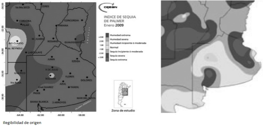
Source: Centro de Relevamiento y Evaluación de Recursos Agrícolas y Naturales
Figure 1 Palmer drought index January 2009 and 20126
Tables 2, 3, 4, 5, 6, and 7 summarize income loss of soybean production at a county level in the Provinces of Buenos Aires, Cordoba, Santa Fe, Entre Rios y La Pampa valued in current dollars.
Table 2 Province of Buenos Aires
| Counties | Income loss 2009 in u$s of current year |
Income loss 2012 in u$s of current year |
|---|---|---|
| 25 de Mayo | 30.18 | - |
| 9 de Julio | 85.08 | - |
| Alsina | 26.98 | - |
| Adolfo Gonzales Chaves | 26.44 | - |
| Alberti | 35.21 | - |
| Arrecifes | 51.37 | - |
| Ayacucho | 0.86 | - |
| Azul | 23.67 | - |
| Balcarce | 13.28 | - |
| Baradero | 31.37 | - |
| Benito Juarez | 11.91 | - |
| Bolivar | 38.94 | - |
| Bragado | 69.16 | - |
| Campana | 3.74 | - |
| Canuelas | 6.14 | - |
| Capitan Sarmiento | 22.48 | - |
| Carlos Casares | 52.17 | - |
| Carlos Tejedor | 68.14 | - |
| Carmeno de Areco | 28.92 | - 11.63 |
| Castelli | 1.02 | - 3.66 |
| Chacabuco | 101.10 | - |
| Chascomus | 7.01 | - |
| Chivilcoy | 61.96 | - |
| Colon | 29.25 | - |
| Coronel Dorrego | 12.83 | - |
| Coronel Pringles | 6.84 | - |
| Coronel Suarez | 35.53 | - |
| Daireaux | 40.34 | - |
| Dolores | 8.45 | - |
| Exaltacion de la cruz | 7.98 | - |
| Florentino Ameghino | 42.58 | - 38.42 |
| General Alvarado | - | _ 5.45 |
| General Alvear | 5.63 | - |
| General Arenales | 51.96 | - |
| General Belgrano | 7.80 | - |
| General Juan Madariaga | 2.98 | - 3.27 |
| General La Madrid | 7.72 | - |
| General Las Heras | 3.23 | - |
| General Pinto | 60.20 | - 33.35 |
| General Pueyrredon | 4.83 | - |
| General Rodriguez | 1.55 | - |
| General Viamonte | 42.09 | - |
| General Villegas | 134.19 | - 88.36 |
| Guamini | 25.21 | - |
| Hipolito Yrigoyen | 17.48 | - |
| Junin | 99.41 | - |
| Laprida | 5.18 | - |
| Las Flores | 10.38 | - |
| Leandro N. Alem | 65.80 | - 33.81 |
| Lincoln | 65.86 | - 44.85 |
| Loberia | 13.71 | - |
| Lobos | 17.36 | - |
| Lujan | 8.52 | - 3.35 |
| Maipu | 10.98 | - |
| Marcos Paz | 5.25 | - |
| Mercedes | 10.41 | - |
| Monte | 9.74 | - |
| Navarro | 13.56 | - |
| Necochea | 15.15 | - |
| Olavarria | 42.08 | - |
| Patagones | 0.06 | - |
| Pehuajo | 91.25 | - |
| Pellegrini | 10.26 | - |
| Pergamino | 96.40 | - |
| Pilar | 1.24 | - |
| Puan | 0.16 | - |
| Ramallo | 43.58 | - |
| Rauch | 34.66 | - |
| Rivadavia | 101.26 | - |
| Rojas | 92.89 | - |
| Roque Perez | 18.31 | - |
| Saavedra | 8.88 | - |
| Saladillo | 20.69 | - |
| Saliquelo | 8.70 | - |
| Salto | 52.79 | - |
| San Andres de Giles | 36.09 | 16.91 |
| San Antonio de Areco | 31.35 | - |
| San Cayetano | 23.23 | - |
| San Nicolas | 29.10 | - |
| San Pedro | 39.79 | - |
| Suipacha | 8.27 | 9.54 |
| Tapalque | 0.66 | - |
| Tornquist | 0.86 | - |
| Trenque Lauquen | 91.66 | - |
| Tres Arroyos | 26.62 | - |
| Tres Lomas | 11.59 | - |
| Villarino | 0.06 | - |
| Zarate | 18.61 | - |
| TOTAL | 2,638.22 | 292.61 |
Source: own elaboration
Table 3 Province of Córdoba.
| Counties | Income loss 2009 in u$s of current year | Income loss 2012 in u$s of current year |
|---|---|---|
| Marcos Juárez | 95.53 | 228.64 |
| Unión | - | 221.32 |
| Rio Cuarto | - | 180.35 |
| San Justo | 86.60 | - |
| General Roca | 131.81 | - |
| Pres.R. Saenz Pena | 115.10 | 107.89 |
| Rio Segundo | - | 234.34 |
| Tercero Arriba | - | 117.20 |
| Rio Primero | 99.33 | 134.78 |
| Juárez Celman | 82.36 | 120.72 |
| Colon | 27.53 | - |
| Rio Seco | 25.92 | - |
| Totoral | 47.24 | - |
| General San Martin | - | 129.28 |
| Tulumba | 35.98 | 40.41 |
| Calamuchita | - | 32.93 |
| TOTAL | 747,4 | 1.547,86 |
Source: own elaboration
Table 4 Province of Santa Fé
| Counties | Income loss 2009 in u$s of current year | Income loss 2012 in u$s of current year |
|---|---|---|
| General Lopez | 175.91 | 240.43 |
| Caseros | 68.60 | - |
| San Lorenzo | 68.17 | - |
| Rosario | 40.80 | - |
| San Justo | 45.34 | 45.60 |
| San Cristobal | 25.73 | 31.05 |
| General Obligado | 15.26 | 25.48 |
| 9 de Julio | 29.30 | 17.24 |
| Belgrano | 41.86 | - |
| Castellanos | 52,75 | 111.69 |
| Constitución | 67.02 | - |
| Las Colonias | 73.52 | - |
| La Capital | 15.44 | - |
| Vera | 4.74 | 9.67 |
| San Javier | 1.94 | 3.02 |
| TOTAL | 727,37 | 484,18 |
Source: own elaboration
Table 5 Province of Entre Rios.
| Counties | Income loss 2009 in u$s of current year | Income loss 2012 in u$s of current year |
|---|---|---|
| Colon | 8.01 | - |
| Concordia | 11.58 | - |
| Diamante | 30.58 | - |
| Federacion | 1.77 | - |
| Federal | 8.62 | - |
| Feliciano | 2.84 | - |
| Gualeguay | 45.15 | - |
| Gualeguaychu | 42.35 | - |
| La Paz | 24.57 | - |
| Nogoya | 48.64 | - |
| Paraná | 55.20 | - |
| San Salvador | 8.46 | - |
| Tala | 16.03 | - |
| Uruguay | 37.53 | - |
| Victoria | 55.33 | - |
| Villaguay | 26.55 | - |
| TOTAL | 423.2 | - |
Source: own elaboration
Table 6 Province of La Pampa
| Counties | Income loss 2009 in u$s of current year | Income loss 2012 in u$s of current year |
|---|---|---|
| Atreuco | 4.27 | - |
| Capital | 2.38 | - |
| Catrilo | 6.68 | - |
| Chapaleufu | 30.33 | - |
| Conhelo | 3.37 | - |
| Maraco | 25.19 | - |
| Quemu Quemu | 10.30 | - |
| Rancul | 2.36 | - |
| Realico | 5.42 | - |
| Toay | 0.04 | - |
| Trenel | 2.33 | - |
| TOTAL | 92.68 | - |
Source: own elaboration
Table 7 Summary
| Province | Income loss 2009 in u$s of current year | Income loss 2012 in u$s of current year |
|---|---|---|
| Buenos Aires | 2,638.22 | 292.61 |
| Córdoba | 747.40 | 1,547.86 |
| Santa Fé | 727.37 | 484.18 |
| Entre Rios | 423.21 | - |
| La Pampa | 92.68 | - |
| Total | 4,628.88 | 2,324.65 |
Source: own elaboration
87 out of 95 counties of the Province of Buenos Aires suffered extreme decreases in yields in 2009, representing a total loss of u$s 2.638 million valued in dollars of that year. However, only 8 out of 95 counties were severely affect by the 2012 drought, with an estimated loss of u$s 292 million.
The Province of Córdoba has a total of 17 counties. In this case, 8 counties have experience extreme decreases in yields in 2009 and 11 in 2012, with a total income loss of u$s 747 million and u$s 1,547 million, respectively.
The Province of Santa Fe has 18 counties and 14 of them suffered extreme decreases in yields in 2009, representing a total loss of u$s 727,3 million valued in dollars of that year. In 2012, 8 out of 18 counties where severely affected, with an estimated loss of u$s 484,18 million.
Lastly, all Entre Rios counties suffered extreme events decrease in yields during 2008/09 campaign and 11 out of 13 counties of La Pampa exhibit the same pattern.
Therefore, the total income loss is estimated in u$s 4.628 million for 2009 and u$s 2.324 for 2012, both figures in current dollars of each year. Calculating the total loss in dollars of 2016 by means of the international risk free rate7, the final estimate is u$s 8.046 million. In relative terms, that amount represent 22% of international reserves of Argentinean Central Bank in 2016.
Discussion
The presented methodology works as follows, if an extreme deviation in yield is detected then the model compare against Palmer Drought Index in order to confirm or dismiss the extreme event. When both conditions are reached, the economic loss is calculated.
Therefore, the methodology only values extreme events, both in relation of the level of decrease in yields and the level of drought. This approach has proven to be robust enough to the objective of valuate the impact over a large geographical area with limited local information.
Regarding the utility of the results, the approach works well enough to conclude that severe and excessive droughts have a macroeconomic impact in the case of Argentina, in contrast with other countries where extreme droughts can have impacts over food security instead of macro-financial effects. This shapes the kind of instruments that should be developed in the climate risk adaptation agenda.
Agricultural economic structure of soybean production is export-oriented and production downturns do not generate homeland problems of food security. Impact on producers might be high, but can be compensated with good weather years, as droughts have not been a trend8. However, macroeconomic and fiscal policy has been procyclical and trade balance highly dependent on commodities exports (Massot, 2016; Sorrentino and Thomasz, 2015). Therefore, macro-fiscal planning can benefit from setting public expenditure and reserves consumption according to the structural behavior of cyclical resources (IMF, 2015; OCDE/CEPAL/CAF, 2015; Ardaz et al, 2015; Schaechter et al, 2012). Despite risk price in soybean has been studied in relation to shocks of American stocks and interest rate shocks (Thomasz, 2016), the effect of internal weather events on country-scale production quantities in Argentina still remain as a question. Therefore, the methodology presented in this study provides the first step to provide an answer to that question. Moreover, despite its own singularities and limitations, the simplicity of the approach makes it easy to be applied to any country and any crop with limited information -all models are wrong, some are useful (Box, 1979)-.
The other limitation is concerning future forecasts. The approach is primarily a methodology of deconstructing the past, but it can be easily adapted as a predictive tool following a stochastic simulation approach. However, even if average production and international prices could be forecast, climate modeling and specially climate variability modeling remains a challenge. As it was said, South Eastern South America (SESA) is a region that has exhibited one of the largest wetting trends during the 20th Century (Barros, 2015; Gonzales, 2014). Climate models suggest that stratospheric ozone depletion results in a significant wetting of SESA over the period 1960-1999 (Gonzales, 2014; Barros, 2015). Since the ozone layer is predicted to recover, precipitation will stabilize or, possibly, decrease in the coming decades (Gonzales, 2014). However, this forecast does not include the incidence and recurrence of severe and extreme drought events, which were the cases presented in this study. As a result, a scenario simulation approach can be presented, which will be one of the main continuation of this line of research.
Conclusions
This paper has presented a simple approach to value past economic losses in soybean production due to cases of extreme or severe drought. Extreme deviations were analyzed and compared with the Palmer Drought Index and by means of the construction of counterfactual of a non-extreme variability scenario, production losses are monetized by means of the international soybean price.
The study was developed at a county level for the Provinces of Buenos Aires, Cordoba, Santa Fe, Entre Rios y La Pampa finding a coincidence between extreme negative deviation in yields and severe and extreme cases of droughts.
In the last 17 years, the agricultural campaigns of 2008/2009 and 2011/2012 suffered the greatest decreased in soybean yields at a county level. The total loss generated in those years was estimated in u$s 8.046 million in 2016 dollars, amount that represents 22% of Argentinean’s international reserves of 2016.
The objective of the estimation is to provide a general approximation of estimated income losses to have a first glance of the dimension of the phenomena, and therefore consider if there is any economic convenience of applying adaptation measures. The case analyzed provides a rapid approach and the magnitude of the estimation -which is conservative because it measures the loss relative to the one standard deviation and not to the mean- permits to conclude that cases of severe and extreme drought might increase macroeconomic risk due to dependence of soybean exports.
Despite the fact that the methodology may have certain limitations, it provides an easy understandable approach to policy makers, it requires basic information and can be easily replicated to other crops. Nevertheless, the estimates must be considered as a starting point of discussion and not as a precise valuation, therefore more into detailed research has to be done depending the kind of adaptation measure to be implemented. For instance, this approach is not adequate to design an index based insurance; on the other hand, might provide insights to design macroeconomic and fiscal stabilization rules.
Future research on this area will complete estimates with the study of the reaction of crops to different levels of drought, as well as the incidence of other events such as excessive rainfall.

