


Serviços Personalizados
Journal
Artigo
 texto em
  Inglês (pdf)
 Artigo em XML
 Referências do artigo
 Enviar este artigo por email
Indicadores
-
 Citado por SciELO
 -
 Acessos
Links relacionados
-
 Similares em
SciELO
Similares em
SciELO
Compartilhar

 Permalink
Contaduría y administración
versão impressa ISSN 0186-1042
Contad. Adm vol.63 no.4 Ciudad de México Out./Dez. 2018
https://doi.org/10.22201/fca.24488410e.2018.1905
Articles
Is there any relationship between the monetary base and the interest rate of the US Federal Reserve?
1Universidad Nacional Autónoma de México, Mexico.
The present paper deals with the United States Federal Reserve (Fed) way of manipulating the interest rate (i) within a framework of endogenous supply of money, exogenous interest rate and inflation targeting. We argue that the Fed controls the monetary base (H) with the aim of adjusting the federal funds interest rate. In order to empirically support our hypothesis, an econometric analysis is conducted with data from the US economy for the period 1990-2017. It is shown that there is a long-run relationship between the fluctuations of both H and i. Furthermore, it is also shown that the volatility of H significantly affects the behavior of i. It appears that this issue has not been sufficiently discussed in the relevant literature, hence -we would like to stressour results represent the main contribution of this study.
Keywords: Monetary base; Monetary supply; Interest rate; Inflation
JEL classification: E51; E43; E31
En este artículo analizamos la forma en que la Reserva Federal de los Estados Unidos (Fed) ajusta la tasa de interés (i) en una economía con oferta monetaria endógena, tasa de interés exógena y objetivos de inflación. Sostenemos la hipótesis de que la Fed manipula la base monetaria (H) para realizar los movimientos de la tasa de interés de los fondos federales. Este problema no ha sido suficientemente estudiado en la literatura relevante y consideramos que representa la aportación fundamental de este estudio. Para documentar nuestra hipótesis, realizamos un análisis empírico con datos de la economía de los Estados Unidos para el periodo 1990-2017. Los resultados muestran que existe una relación de largo plazo entre las fluctuaciones de H e i. Además, se observa que la volatilidad de H influye significativamente en el comportamiento de i.
Palabras clave: Base monetaria; oferta monetaria; tasa de interés; inflación
Códigos JEL: E51; E43; E31
Introduction
The current framework of monetary policy of the United States Federal Reserve (Fed) is based on the thesis of the New Consensus in Macroeconomics (NCM), which states that a low and stable inflation regime is conducive to optimal growth and full employment (Taylor, 1993; Bernanke et al., 1999; Bernanke and Mishkin, 1999; Clarida et al., 2001). In this paradigm of monetary policy, the interest rate is the only instrument of the central bank (CB) to achieve price stability, and there are no intermediate goals. The interest rate (i) is exogenous and, therefore, the money supply (M) is endogenous.The CB manipulates i in response to fluctuations of both inflation and output. How does the CB carry out these interest rate movements?
Regarding M there are two approaches: the theory of monetary exogeneity and the theory of the endogeneity of money supply. The first, formulated mainly by Milton Friedman (1956, 1968), asserts that the CB exogenously controls the quantity of money in the economy, regardless of financial markets; the second postulates that the CB does not control M, as the money supply is determined within the financial system (cf. Wicksell, 1898; Kaldor, 1982; Moore, 1988). According to the theory of monetary exogeneity, the CB aims to achieve price stability by defining growth targets of some monetary aggregate. On the other hand, interest rate objectives determine price stability in the theory of monetary endogeneity.
Since the 1990s, a growing number of central banks have abandoned monetary aggregates as an instrument for their policy and, instead, interest rates have become the reaction function of the monetary authority to achieve the inflation target. Again, this implies that control of inflation depends on the movements of i. The question that arises from this discussion is how the adjustments of the interest rate come about in a monetary policy framework of inflation targeting with an endogenous money supply.
The purpose of this article is to analyze the operational mechanism by which the CB moves the interest rate to reach the selected inflation target. Our hypothesis is that, in an economy with endogenous M and exogenous interest rates, the central bank manipulates the monetary base (H) with the aim of adjusting i. In order to contrast our argument, we conducted an econometric analysis based on empirical evidence from the US economy for the period of 1990-2017, a period during which the Federal Reserve (Fed) has followed an inflation targeting monetary policy framework.We also considered two sub-periods, 1990-2000 and 2001-2017. The choice of the US economy for our empirical analysis is justified not only by the unquestionable importance of the Federal Reserve for international monetary policy, but also by the fact that interest rate movements of the federal funds of the Fed impact on both other central banks’ monetary policy and global financial markets. Additionally, the monetary base of the Fed is the lever used to carry out interest rate movements.
The endogeneity of M has been widely discussed in the relevant literature and there is consensus on the direction of causality from demand to supply and from credit to deposits (Lavoie, 2014). However, the matter of whether the CB moves H to control i has received less attention. The specific contribution of this article is to scrutinize the relationship between the fluctuations of H and those of i.
After this introduction, we present a brief review of the debate on monetary endogeneity and continue with the discussion of some stylized facts on the behavior of the monetary variables of our analysis. We then report the results of the empirical contrast conducted with data from the US economy. The article is closed with a conclusion.
Monetary endogeneity: a brief review of the debate
The theory of endogenous money supply maintains that the demand for money and credit determines the supply. In opposition to the modern quantity theory of money by Milton Friedman and other monetarist authors (Friedman, 1956, 1968; Friedman and Schwartz, 1969; Goodfriend, 1997) this theory rejects the existence of a causal relation from the quantity of money towards the level of prices. There are two approaches to the endogeneity of M: neoclassical theory or New Consensus of Macroeconomics (NCM) and Post-Keynesian theory (PKT). Both share some premises for analysis and differ in terms of the role of the financial system and the mechanisms for transmitting monetary policy to prices and economic activity in general.
The NCM determines i based on the reaction function of the central bank; the effect of the movements of i on the price level, output, and employment flows through savings and inter-temporal consumption; financial markets are simple intermediaries facilitating credit creation and reducing transaction costs; and money is a neutral medium of exchange in the long-term.
Post-Keynesian theory, on the other hand, argues that the CB controls the nominal interest rate, and the effects of this on inflation and economic activity take place through investment and income distribution (Moore, 1988; Lavoie, 2014). Since money is defined as a debt and credit instrument, monetary policy is not neutral. Nicholas Kaldor (1970), one of the most important pioneers of monetary endogeneity, maintains that the postulates based on quantity theory are anachronistic and inadequate in economies where money is essentially fiduciary, and the banking system is a source of creation and destruction of money. In these circumstances, demand determines the supply of credit and it is impossible for there to be an excess supply of money. Kaldor (1982: 22) explains it as follows:
“A theory of the value of money based on an economy of commodity money is not applicable to an economy of credit money. In the former, money has an independent supply function based on production costs, whereas in the latter, new money is created from an extension of bank credit. If more money is created as a result-given a level of income or expenditure-the desire to own will automatically eliminate the excess of money.”
Kaldor’s argument implies that the amount of money is endogenously adjusted to the decisions of the public according to the need to finance consumer spending, investment, and the refinancing of outstanding debt. In general terms, this analysis emphasizes three fundamental aspects: first, the price level and inflation correspond to a supply process, not a demand one; second, the greater importance of fiduciary money vis-à-vis commodity money; and third, the role of credit as a central element for the analysis of money supply and demand. Kaldor’s approach inspired the development of the heterodox theory of money. In this theory, two interpretations of the endogeneity of the money supply coexist: the accommodationist or horizontalist and the structuralist views. We will now comment on its fundamental theses.
Horizontalist endogeneity
The authors of the “accommodationist” position argue that there are no quantitative restrictions on bank reserves.The decisions of the financial system generate an endogenous expansion of the amount of money (cf. Kaldor, 1982; Lavoie, 1985; Moore, 1988, 1991; Goodhart, 1989; Pollin, 1991; Palley, 1996; Rochon, 2001). Unlike the IS-LM model (cf. Hicks, 1937), the accommodationists represent the money supply as a horizontal line, since monetary policy is expressed with a given interest rate, not as a fixed amount of money: demand determines supply.1
The foregoing means that commercial banks can always obtain additional reserves at a given price, provided that confidence in their solvency is maintained; as a result, solvent banks are never quantitatively constrained at obtaining reserves. The money supply function is horizontal, given an interest rate that depends on the price of the marginal supply that the monetary authority sets for the reserves. In this sense, the monetary policy instrument is the short-term interest rate. Moore (1988), in turn, emphasizes the non-discretionary nature of bank reserves; the causal relationship runs from loans to deposits and deposits create reserves. The central argument is that private decisions made by banks and their customers determine the supply of loans and deposits, causing the credit supply to expand endogenously to meet the exchange needs of the agents. The central bank can only fix the short-term interest rate at which it offers reserves.
The horizontalist approach has two central arguments, the first concerning the loan/reserve/deposit ratio and the second concerning how the interest rate relates to this ratio. The first notion (loans determine monetary aggregates) is opposed to the direction of causality (from monetary aggregates to credit) set by monetarism. The second argument refers to the fact that the CB can determine the behavior of short-term interest rates. This power derives from two sources: from the control of the monetary authority over the discount rate and from the control of the short-term interest rate through open market operations (OMOs) with which commercial banks obtain resources from the CB. Once it sets directly the discount rate, and indirectly the short-term rate, the market interest rates move accordingly (Pollin, 1991:370).
Under the horizontalist approach, the CB imposes quantitative restrictions on reserves: when commercial banks do not have sufficient deposits to meet reserve requirements, they must make up for any shortfall by borrowing from other banks-either through the sale of assets or by borrowing directly from the CB. Although the central bank may determine the amount of non-loanable reserves, these are not equal to the total reserves required, which means that they are not under the strict control of the monetary authority. If banks have to collect a certain amount of required reserves, the CB has no choice but to provide the total volume of reserves for the banking system at a given price (Moore, 1988: 374).
In empirical terms, Moore (2001) states that the problem is multiple, since it can be observed that the series of reserves, deposits, and loans move together (see also Rochon and Rossi, 2003). The empirical question is to determine the causal relationship between reserves and deposits. However, it is very difficult to establish this direction of causality, which is why the hypothesis of the endogeneity of money is not always accepted by orthodox economists. In short, Moore (1988:12) suggests that, when reviewing the time series and performing the econometric techniques, it should be considered that: the credit supply is determined by the demand for bank credit; the causality is predominantly from bank loans to deposits and from there to H; and, finally, the short-term interest rate-the instrument of the monetary policy-is determined exogenously.
Structuralist endogeneity
The structuralist approach to endogenous money suggests that the monetary authority and the banks themselves do not follow a completely comfortable behavior, that is, M is partially exogenous (Rochon, 2003:133). The CB also makes policy decisions based on its balance sheet; for example, when the overall price level is high (low), the CB is less (more) willing to allow an increase in demand for reserves. That is, it may prefer to raise the short-term interest rate to encourage commercial banks to reduce their lending activity. The effects on M are explained according to the liquidity preference theory. For structuralists, the supply of monetary reserves and credit are represented by positive sloping curves (Fontana, 2003).
The CB moves i in response to changes in demand for currency reserves and is not necessarily willing to offer all the demanded reserves at a fixed price. Unlike horizontalists, structuralists say, the possibility of other sources of variation of the differentials of interest rates dissimilar to those of the influence of the CB is opened.
A key point of the structuralist authors (difficult to prove empirically) is that the counter-cyclical monetary policy is not only denoted by an increase (decrease) of the interest rate in periods of boom (recession), but that the amount of money of the CB controls the supply of reserves of the banking system, which means a quantitative rationing without price as a way of not revealing the level of the short-term interest rate (Moore, 2001).
On the other hand, the direct relationship between the demand for credit and the interest rate on loans is explained by structuralists following the approach by Hyman Minsky regarding the behavior of financial corporations. Most structuralists argue that banks raise their bencnhmark interest rates at the height of the economic cycle, as credit rises, banks become concerned about their portfolio balance as well as the liquidity levels of their clients (Fontana, 2001: 373).
Additionally, some structuralists analyze other factors that trigger endogenous variations in market interest rates. One of the explanations is found in the liability management carried out by banks when the resources obtained from the CB are very costly. This management is what provides the necessary reserves that support the decision of the banks to “lend first and then find the reserves”. In general terms, liability management is the search for funds-other than deposits-that do not have high reserve requirements in the money market. These types of practices within financial innovations can help meet the reserve needs of the system, but they are costly to develop because they tend to transfer funds from liabilities with high reserve requirements and low cost to liabilities with low reserve requirements and high cost, which makes intermediation more expensive and raise the interest rates (cf. Pollin, 1991:375).
Structuralists argue the importance of including the effects of the preference for liquidity in the analysis of money. These effects are the result of incorporating the portfolio decisions of wealth holders who, for precautionary or speculative reasons, distribute their income between liquid deposits and other financial assets such as bonds, stocks, securities, among others. For structuralists, these portfolio options cannot be separated from the interest rate differentials, given that the changes in these are part of the intricate portfolio adjustments whose effects are relevant in the transmission process of the monetary policy (cf. Fontana, 2001:375).
These characteristics are the result of institutional changes associated with the development of the banking system. For example, in the early historical stages of banking, money was exogenous, and banks acted as pure financial intermediaries, in accordance with the analysis of neoclassical theory (causality of deposits-reserves-lending). The credit supply was pre-determined and the principle of scarcity was valid. However, when the CB becomes the agency responsible for the stability of the financial system, commercial banks can expand loans beyond their reserve capacities. This is the ‘accommodative’ function of the CB, i.e., the removal of reserve restrictions that are part of the endogenous nature of the money supply (Rochon, 2003:132).
In short, the recent development of the financial system-mainly due to the process of financial innovation, globalization, technological advances, and institutional changes-has not only modified the placement, rating, and trading of financial assets, but has also altered the way in which economic agents finance themselves and the modus operandi of credit supply and demand. In terms of the horizontalist approach, it can be seen as a less extreme version of the endogeneity of money, where banks actively pursue financial innovations in order to expand the supply of credit. In terms of the structuralist approach, these financial metamorphoses reinforce the role of the preference for liquidity.2
Stylized facts of monetary variables
Following the debate on the endogeneity of money, we present below some stylized facts reflecting the monthly evolution of the monetary variables of the United States economy over the period 1990-2017. The next figures give a general idea of how the inflation targeting monetary policy has operated in the most important economy in the world. Figure 1 shows the growth of the money supply (represented by the monetary aggregate M2),whose behavior remains stable during the first years of the adoption of the inflation targeting regime. It is since the dot.com crisis of 2000/01 when a high volatility of M2 is observed, which deepens with the 2007/08 crisis. With the adoption of the quantitative easing policy, the Fed pursues a policy of restricted discretion, which is reflected in the periodic fluctuations of M.
Source: own elaboration with data from FRED, 1990-2017.
Figure 1 Behavior of the money supply. United States, 1990-2017.
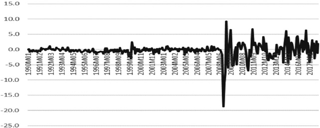
Figure 2 shows the variations of the total monetary base, which remained stable until the crisis of 2000/01, when H presented imbalances (-0.040 and 0.019). After the dot.com crisis, the Fed reduced the interest rate of the federal funds (iff) in order to stimulate the economy, a decision reflected in the stabilization of H. Since the subprime crisis of 2007/08, significant fluctuations and outliers have been observed. This destabilizing behavior as of 2010 is associated with the adoption of an interest rate close to zero. Therefore, it is recognized that in circumstances of a restricted monetary policy, H acts as an exogenous variable to stabilize i and thus achieve monetary stability (Anderson, 2009; Gavin, 2009).
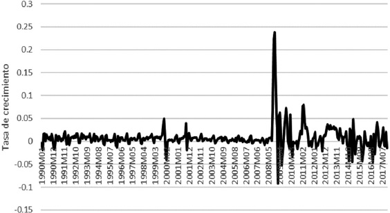
Source: own elaboration with data from FRED, 1990-2017.
Figure 2 Behavior of the monetary base. United States, 1990-2017.
Figure 3 shows the trajectory of iff. As with the previous variables, iff shows a stable behavior during the first years of the adoption of the Taylor rule to achieve low and stable inflation. However, as a result of the 2000/01 crisis, the Fed reduced iff, its monetary policy instrument, to levels below 2% in order to revive the economy. Subsequently, in 2005 the Fed decided to gradually raise it until the bursting of the subprime bubble in 2007, when the iff was set at levels very close to zero percent-the so-called zero lower bound-, a policy stand maintained until early 2016, when the Federal Open Market Committee (FOMC) initiated the “normalization” of monetary policy by slowly and marginally increasing the iff (Bernanke, 2009; Aubuchon, 2009).
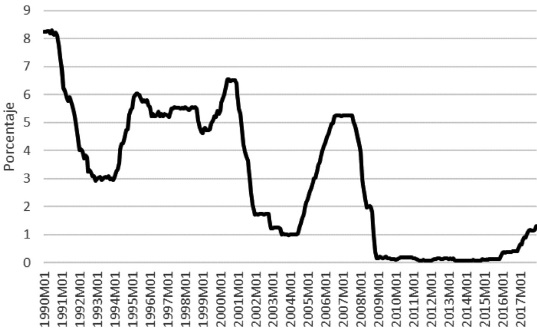
Source: own elaboration with data from FRED, 1990-2017.
Figure 3 Behavior of the federal funds interest rate. United States, 1990-2017.
Given that iff is an exogenous variable used to reach an inflation target, it is relevant to compare the behavior of the former vis-à-vis the latter. Figure 4 shows how the CB has achieved low and stable inflation. It is even possible to observe an indirect relationship until the early 2000s. As a result of the aforementioned crises and the subsequent decisions of the Fed to temporarily abandon the Taylor rule, the interest rate does not seem to have had an impact on inflation, as it remains stable while i stays at levels close to zero percent. Therefore, the short-term interest rate seemed to have lost its effectiveness, which raised the question of whether it still works as an optimal instrument.
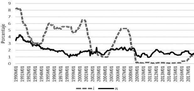
Source: own elaboration with data from FRED, 1990-2017.
Figure 4 Behavior of the interest and inflation rates. United States, 1990-2017.
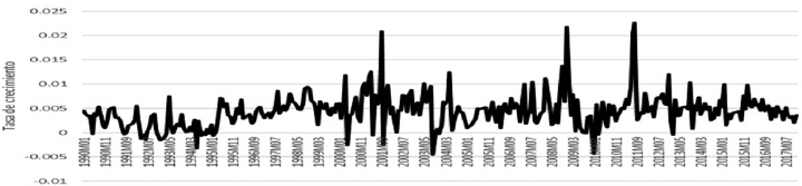
The main reason for reducing the interest rate in post-crisis periods was to reinvigorate the economy by stimulating the components of aggregate demand. However, the US economy in real terms during the period under review shows a tendency towards stagnation. Figure 5 shows that output has not reached pre-crisis levels, even though the level of the interest rate remains very low by historical standards. It seems clear that during the life of the monetary policy model inspired by the NCM, i-the instrument par excellence of monetary policy-has also lost its effectiveness.
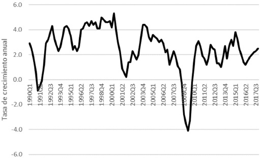
Source: own elaboration with data from FRED, 1990-2017.
Figure 5 GDP growth rate. United States, 1990-2017.
The behavior of i with respect to inflation and output shows that the Fed has not followed a monetary policy rule, but rather a policy framework of pragmatic discretion (Bernanke calls it restricted discretion). It has abandoned the interest rate as the anchor of inflation, as opposed to the NCM canon. The behavior of the interest rate observed during the period under analysis shows that in crisis episodes, it moves away from the reaction function estimated by the Taylor rule and, therefore, loses effectiveness. This can be corroborated by observing the period 2002-2005: after the dot.com crisis, the Fed decided to reduce the interest rate below the level recommended by the policy rule. Taylor (2007) argues that this decline in interest rates provided large amounts of liquidity, thus helping to promote speculation with financial assets and in the real estate market with a marked increase in demand for housing. Taylor criticizes the Fed´s decision of low interest rates maintained over a long period of time, which encouraged asset price inflation associated with the mortgage market, and thus a new financial bubble.
After the subprime crisis, Bernanke (2015) took up this criticism and estimated a Taylor rule. The result shown in this study is that for the post-crises periods (2001 and 2008), the Taylor rule recommends reducing the interest rate even below the observed level, even considering negative levels. Therefore, Bernanke argues that the Fed acted systematically, not automatically, by making the best monetary policy decisions ever.
If the Fed has acted with restricted discretion, keeping its policy instrument at very low levels, it is very important to analyze which variable has been manipulated to reach that interest rate target. Figure 6 shows the elasticity between M and i, that is, the ratio coefficient between M and i. The sensitivity of M to changes in i becomes very volatile during and after the subprime crisis, indicating an adjustment of M to keep the interest rate low and stable. However, this behavior is not typical of a post-crisis period, given that after the abandonment of monetary aggregates as an instrument for monetary policy and the adoption of the Taylor rule, the volatility observed between both variables is implicit.
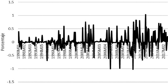
Source: own elaboration with data from FRED, 1990-2017.
Figure 6 Elasticity between the money supply and the interest rate. United States, 1990-2017.
On the other hand, as shown in Figure 7, the fluctuations of the elasticity of H, the monetary base (before changes in i), and the interest rate are a post-crisis phenomenon. When observing a great volatility and that the interest rate was kept at very low levels, it is possible to suppose that H has been the adjustment variable for moving the interest rate to reach the desired price level.
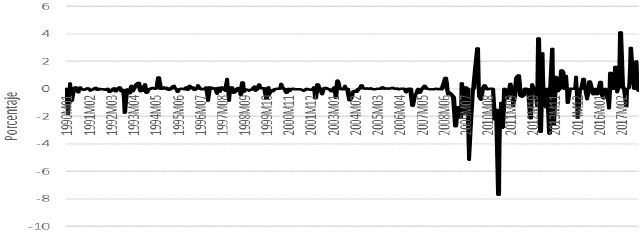
Source: own elaboration with data from FRED, 1990-2017.
Figure 7 Elasticity between the monetary base and the interest rate. United States, 1990-2017.
Similarly, it is important to observe the behavior of the money multiplier, calculated as the coefficient between the monetary aggregate M1 and H3. Figure 8 shows that the strong fluctuations of this variable occurred after the crisis of 2007/08. This behavior corroborates what is observed in Figure 7. In other words, H acts as an exogenous variable in order to move the interest rate.
Source: own elaboration with data from FRED, 1990-2017.
Figure 8 Behavior of the money multiplier. United States, 1990-2017.
After considering the above stylized facts, it is necessary to prove the causal relationship between i and H. We wish to analyze the matter of whether the Fed manipulates H to control i and thus achieve the objective postulated by NCM.
Empirical analysis
We proceed to establish the relationship between the fluctuations of the interest rate and the monetary base as follows:
Where i is the federal funds interest rate, H is the total monetary base, and ε t is an error term. To analyze the long-term relationship between the monetary policy instrument and the monetary base, we intend to identify equation (1) in a long-term structure of a cointegrated model, as well as analyze its causal relationship. Our econometric analysis considers monthly data from the St. Louis Federal Reserve database of the involved variables for the period 1990-2017. The monetary base is considered in logarithms and both variables are used in terms of their first difference. To determine whether CVAR is the best model to empirically estimate equation (1), it is necessary to perform the unit root test to identify whether the variables are stationary. The results of the test (see Table 1) show that both variables are of order of integration I (0).
Table 1 Unit Root Test with the augmented Dickey-Fuller test.
| Model | |||
|---|---|---|---|
| Variable | Intercept | Trend and intercept | None |
| I | -2.5441 | -3.0856 | -2.1738 |
| LH | 0.1210 | -1.6849 | 3.5113 |
| ∆I | -5.3996 | -5.4579 | -5.3557 |
| ∆LH | -10.9684 | -10.9742 | 10.2183 |
Note: ∆ indicates the first difference of the series. The level of significance is 5%
Source: own elaboration with data from FRED, 1990-2017.
From this identification it can be concluded that the CVAR is the appropriate model for estimating long-term coefficients. The first stage of the method is to calculate the Vector Autoregression (VAR). It can be seen that the VAR model is not consistent for the whole sample due to the presence of outliers, 2008/09, found in Figure 2. Therefore, given the fluctuations of the variables, we cut the sample into two sub-periods, 1990-2000 is the first sub-period and 2001-2017 the second. With regards the first period, the appropriate VAR model for equation (1) is given with 8 lags. The lags were selected in accordance with the general diagnosis of the model. Also, a good model specification is accepted, i.e., the residuals are normal, homoscedastic, and there is no evidence of serial correlation (see Tables A and B in the statistical appendix).
The second stage is the transformation of the VAR into a cointegrated model (CVAR). The Johansen methodology is used to find out if the variables in equation (1) are cointegrated. The results of this test are shown in Table 2. It can be seen that, according to the Trace and Maximum Eigenvalue tests, there are two cointegration vectors for each type of test.
Table 2 Johansen cointegration test
| Data trend | None | None | Linear | Linear | Quadratic |
| Type of test | No intercept | Intercept | Intercept | Intercept | Intercept |
| No Trend | No Trend | No Trend | Trend | Trend | |
| Trace | 2 | 2 | 2 | 2 | 2 |
| Max-Eig | 2 | 2 | 2 | 2 | 2 |
| Data trend | None | None | Linear | Linear | Quadratic |
| No Intercept | Intercept | Intercept | Intercept | Intercept | |
| Type of test | No Trend | No Trend | Trend | Trend | Trend |
| Trace | 2 | 2 | 2 | 2 | 2 |
| Max-Eig | 2 | 2 | 2 | 2 | 2 |
Note: critical values at 0.05 significance based on MacKinnon-Haugh-Michelis (1999).
Source: own elaboration with data from FRED, 1990-2000.
The normalized cointegration vector was selected at a 0.05 level of significance and according to the best relations in economic terms (with intercept and trend).
Table 3 shows the estimated cointegration vector. In this equation, it is observed that the fluctuations of the monetary base have a negative influence (-0.22) in the variations of the interest rate. This means that an increase (decrease) in the monetary base reduces (increases) interest rate changes. Once we have verified that there is a long-term relationship for the first cut of the sample, we proceed to analyze whether this relationship found between both variables implies causality. Granger (1969) was the first to propose a causality test for two variables (time series), X and Y; X is said to cause Y in a Granger sense if Y can be better predicted using past information from X and Y than if we only use past information from Y.
We can evaluate the absence of Granger causality estimating the following VAR model:
Based on equations (2) and (3), we carried out causality tests and obtained the results shown in Table 4.
Table 4 Granger causality test
| Dependent variable: I | |||
| Excluded | Chi-q | Df | Probability |
| LH | 15.9995 | 8 | 0.0424 |
| Dependent variable: LH | |||
| Excluded | Chi-q | Df | Probability |
| I | 13.0034 | 8 | 0.1117 |
Note: Significance at 5%
Source: own elaboration with data from FRED, 1990-2000.
With 8 degrees of freedom and a significance level of 5%, the upper panel of Table 4 shows that the null hypothesis of non-causality in a Granger sense from H to i is rejected, while in the lower panel we can observe that the null hypothesis of non-causality from i to H is not rejected. In short, we found causality from the monetary base to the interest rate, but not vice versa.
Regarding the second period (2001-2017), the evidence for finding a long-term relationship is unconvincing. Given the outliers of the do.tcom and subprime crises found in the monetary base data, as well as the structural changes in the interest rate, the realization of a CVAR becomes complex. In the tests there are specification errors, lack of normality in the residues, and heteroscedasticity. Therefore, this method is not suitable for analyzing the relationship of these variables in the established period.
Given the volatility observed in the variables, an alternative model can be a generalized autoregressive conditional heteroscedasticity (GARCH) model, which extends the class of ARCH models (Bollerslev, 1986). In these, the structure of the conditional variance depends, in addition to the square of the delayed errors q periods as in the ARCH(p) model, on the delayed conditional variances q periods (Casas and Cepeda, 2008).The identification of p and q is conducted as in the ARIMA models. Given this information, we developed a GARCH model to observe how the volatility of the monetary base explains the behavior of the interest rate.
We proceeded to perform an ordinary least square (OLS) regression. The result of this test indicates that the monetary base maintains a negative relationship (-0.0184) with the interest rate (see Table C in the statistical appendix). Subsequently, we verified that the model is well specified. In the Statistical Appendix, Table D shows that there is an incorrect specification of the model, given that there is heteroscedasticity, serial autocorrelation, and lack of normality in the residues. To solve these problems with the residuals, we set up a GARCH(p,q) model that was more suitable for our data. Considering GARCH = C(2) + C(3) * RESID(-1)2 + C(4) * GARCH(-1) and a possible lack of normality in the residuals, we used the Bollerslev-Wooldridge covariance method. The best resulting model is a GARCH (1,1).
Table 5 shows the results of GARCH (1,1). The variance of the monetary base exhibits a negative relationship (-0.0045) with the variations of the interest rate. We also observed that the sum of the parameters of the ARCH (.2357) and GARCH (0.7978) structures is very close to 1, which indicates that volatility shocks are quite persistent. Both structures have reliable significance. Regarding the model specification, the heteroscedasticity test shows an F statistic of 0.5988, that is, there is no conditional heteroscedasticity. On the other hand, the correlogram and its probabilities indicate the absence of serial correlation of the residues (see Figure e in the Statistical Appendix). The normality of the residues is non-existent even assuming a Student t-distribution and/or generalized errors. We consider that the model is well specified in most of the tests and since we intend to demonstrate the analysis of the variance of the variables, it is not always possible to achieve the normality of the residues.
Table 5 GARCH (1,1)
| Variable | Coefficient | Probability |
|---|---|---|
| DLH | -0.0001 | 0.0027 |
| Variance equation | ||
| C | 0.0001 | 0.1797 |
| RESID(-1)^2 | 0.2357 | 0.0057 |
| GARCH(-1) | 0.7978 | 0.0000 |
Note: Significance at 5%
Source: own elaboration with data from FRED, 2001-2017.
Therefore, the results for the second sub-period dealt with in the present empirical analysis reveal that part of the volatility of the federal funds interest rate depends on the volatility of the monetary base. Consequently, it can be argued that the monetary base is an exogenous variable used by the Fed to lead the variations of the short-term interest rate.
In general terms, given the results of both the 1990-2000 and 2001-2017 sub-periods, it is possible to test our hypothesis: The Fed manipulates the monetary base to adjust the interest rate. The long-term relationship found in the first years of the application of the inflation targeting regime shows that i is manipulated through H variations in order to achieve the interest rate objective consistent with price stability. Meanwhile, the study of the second sub-period confirms the cointegration relationship. Despite the econometric difficulties and the outliers found in the series, the GARCH model indicates that both the fluctuations of the interest rate and its stability at a level close to zero percent are due to the volatility of the monetary base, the behavior of which, in turn, shows that this is the variable the Fed has been using to perform the movements of the interest rate with the aim of achieving the selected price stability.
Conclusion
Given that several CBs abandoned the objectives of monetary aggregates and instead adopted the nominal interest rate as the primary instrument of monetary policy to control inflation and achieve price stability, the theory of monetary endogeneity has displaced the exogenous theory of the money supply, both in theoretical analyses and in the practice of monetary policy. The predominant monetary policy framework assumes that the money supply is endogenous and the interest rate exogenous. The Fed adjusts the interest rate in response to both deviations of the observed inflation rate with respect to the inflation target consistent with price stability and fluctuations in the gap between observed output and potential output.
Empirical studies analyzing the reaction function of the central bank are abundant, documenting the endogenous nature of the money supply and the interest rate adjustments to control inflation. However, the operational way in which the CB adjusts the interest rate has received less attention from analysts. In this article, we have set out to study precisely how the Fed adjusts its interest rate in an economy with an endogenous money supply, exogenous interest rates, and inflation targets. For this purpose, we support the hypothesis that the CB (in our case, the Fed) manipulates the monetary base to carry out the movements of the interest rate.
To document our hypothesis, we conducted an empirical analysis with data from the US economy for the period of 1990-2017. The empirical evidence led us to the following fundamental result, which constitutes the most important specific contribution of our study: there is a long-term relationship between the fluctuations of the monetary base and those of the nominal interest rate. In addition, we found that the volatility of the monetary base significantly influences the behavior of the nominal interest rate. Therefore, it seems reasonable to conclude that the Fed uses H to adjust the interest rate-its monetary policy instrument-in order to achieve price stability. Finally, we contend that this finding contributes to clarify the role of the monetary base in a monetary policy framework of inflation targeting. This result, that is, the exogenous adjustments of H, is consistent with the hypothesis of the endogeneity of the money supply.
REFERENCES
Anderson, R. (2009). The Curious Case of the U.S. Monetary Base. Federal Reserve Bank of St. Louis Economic Synopses. Available at: https://www.stlouisfed.org/Publications/Regional-Economist/ . Unloaded: 07/02/18 [ Links ]
Aubuchon, C P. (2009). The Fed’s Response to the Credit Crunch. Federal Reserve Bank of St. LouisEconomic Synopses, No. 6. https://doi.org/10.20955/es.2009.6 [ Links ]
Bernanke, B. (2009). The Crisis and the Policy Response. Delivered at the Stamp Lecture, London School of Economics, London, England, January 13. [ Links ]
Bernanke, B. (2015). The Taylor Rule: A benchmark for monetary policy. Available at: https://www.brookings.edu/blog/ben-bernanke/2015/04/28/the-taylor-rule-a-benchmark-for-monetary-policy/ . Unloaded: 07/02/18 [ Links ]
Bernanke, B, Laubach,T, Mishkin, F & Posen, A. (1999). Inflation Targeting, Princeton: Princeton University Press. [ Links ]
Bernanke, B & Mishkin, F S. (1997). Inflation Targeting: A New Framework for Monetary Policy? Journal of Economic Perspectives, 11(2), 97-116.https://doi.org/10.3386/w5893 [ Links ]
Bollerslev, T. (1986). Generalized autoregressive conditional heteroskedasticity. Journal of Econometrics, 31(3), 307-327. https://doi.org/10.1016/0304-4076(86)90063-1 [ Links ]
Casas, M & Cepeda, E. (2008). Modelos ARCH, GARCH Y EGARCH: Aplicaciones a series financieras, Cuadernos de Economía, 27(48), 287-319. [ Links ]
Clarida, R, Gali, J & Gertler, M. (2001). Optimal monetary policy in open versus closed economies: an integrated approach. American Economic Review, 91(2), 248-252. https://doi.org/10.1257/aer.91.2.248 [ Links ]
Fontana, G. (2001). Rethinking Endogenous Money: A Constructive Interpretation of the Debate between Horizontalists and Structuralists. Metroeconomica, Vol. 55, núm. 4, 367-385. https://doi.org/10.1111/j.1467-999x.2004.00198.x [ Links ]
Fontana, G. (2003). Endogenous money: An analytical approach. Scottish Journal of Political Economy, Vol. 50, núm.4, 398-416. https://doi.org/10.1111/1467-9485.5004003 [ Links ]
Friedman, M. (1956). The Quantity Theory of Money, en Studies in the Quantity Theory of Money, Chicago, University of Chicago Press. [ Links ]
Friedman, M. (1968). The Role of Monetary Policy. American Economic Review, 58(1), 1-17. [ Links ]
Friedman, M & A J Schwartz. (1969). The Definition of Money: Net Wealth and Neutrality as Criteria. Journal of Money, Credit and Banking, Vol. 1, no. 1, 1-14. https://doi.org/10.2307/1991373 [ Links ]
Gavin, W T. 2009. More Money: Understanding Recent Changes in the Monetary Base. Federal Reserve Bank of St. Louis Review, March/April 2009, Vol. 91, no. 2, pp. 49-60. https://doi.org/10.20955/r.91.49-60 [ Links ]
Goodfriend, M. (1997). Monetary Policy comes of Age: A 20th Century Odyssey. Federal Reserve Bank of Richmond Economic, Quarterly Volume 83/1 Winter. [ Links ]
Hicks, J R. (1937). Mr Keynes and the “Classics”: A Suggested Interpretation. Econometrica, Vol. 5, no. 2, April, 147-159. https://doi.org/10.2307/1907242 [ Links ]
Kaldor, N. (1970). The new monetarism. Lloyds Bank Review, July, 1-17. [ Links ]
Kaldor, N. (1982). The Scourge of Monetarism, Oxford, Oxford University Press. [ Links ]
Lavoie, M. (1985). The Dynamic Circuit, Overdraft Economics, and Post-Keynesian Economics, en Jarsulic, M., ed., Recent Economic Thought Series. Money and Macro Policy, East Lansing, Michigan, Springer Science+ Business Media LLC. [ Links ]
Lavoie, M. (2005). Monetary base endogeneity and the new procedures of the asset-based Canadian and American monetary systems. Journal of Post Keynesian Economics, Vol.27, no. 4, pp.689-709. [ Links ]
Lavoie, M. (2014). Post-Keynesian Economics: New Foundations. Cheltenham, R.U.-Northampton, MA, Edward Elgar. [ Links ]
Lopreite, M. (2014). The Endogenous Money Hypothesis: An Empirical Study of the Euro Area (1999-2010), Journal of Knowledge Management, Economics and Information Technology, Vol. IV, no. 4, August. https://doi.org/10.2139/ssrn.2084197 [ Links ]
Moore, B J. (1988). Horizontalists and Verticalists, Cambridge, Cambridge University Press. [ Links ]
Moore, B J. (1991). Money supply endogeneity: ‘reserve Price setting’ or ‘reserve quantity setting’. Journal of Post Keynesian Economics, Vol. 13, no.3, 404-413. https://doi.org/10.1080/01603477.1991.11489857 [ Links ]
Moore, B J. (2001). Some Reflections on Endogenous Money. In Rochon, L. P. and Vernengo, M, ed., Credit, Interest Rate and the Open Economy, U.K. Edward Elgar Publishing. [ Links ]
Palley, Thomas I. (1996). Accommodationism versus Structuralism: Time for an Accommodation. Journal of Post Keynesian Economics, Vol. 18, no. 4, 585-594. https://doi.org/10.1080/01603477.1996.11490088 [ Links ]
Pollin, R. (1991). Two theories of money supply endogeneity: some empirical evidence. Journal of Post Keynesian Economics, Vol. 13, no. 3, 366-396. https://doi.org/10.1080/01603477.1991.11489855 [ Links ]
Rochon, L P. (2001). Horizontalism: Setting the Record Straight. In Rochon, L P and Vernengo, M, ed., Credit, Interest Rate and the Open Economy, U.K. Edward Elgar Publishing. [ Links ]
Rochon, L. (2003). On Money and Endogenous Money: Post Keynesian and Circulation Approaches. In Rochon, L P and Rossi, S. 2005. Modern Theories of Money. The Nature and Role of Money in Capitalist Economies, Cheltenham, U.K. Edward Elgar Publishing. [ Links ]
Taylor, J B. (1993). Discretion versus policy rules in practice. Carnegie-Rochester Conference, series on Public Policy 39. North-Holland. [ Links ]
Taylor, J B. (2007). Housing and Monetary Policy, NBER Working Paper no. 13682/07, National Bureau of Economic Research, Cambridge, MA. [ Links ]
Wicksell, K. [1898] (1965). Interest and Prices, Nueva York: Augustus Kelley. [ Links ]
Statistical appendix
Table A Correct specification test- CVAR.
| Test | Statistic | Probability |
|---|---|---|
| Normality | 7.0355 | 0.1340 |
| Heterocedasticity | 117.7721 | 0.0651 |
Note: Significance at 5%
Source: own elaboration with data from FRED, 1990-2000.
Table B Correct specification test- Autocorrelation- VAR.
| Lag | LM-Stat | Probability |
|---|---|---|
| 1 | 2.01957 | 0.7322 |
| 2 | 11.48013 | 0.0217 |
| 3 | 2.85993 | 0.5815 |
| 4 | 11.37076 | 0.0227 |
| 5 | 2.02964 | 0.7303 |
| 6 | 3.95650 | 0.4119 |
| 7 | 0.48082 | 0.9753 |
| 8 | 5.76716 | 0.2172 |
Note: Chi-squaredwith 4 differences.
Source: Own elaboration with data from FRED, 1990-2000.
Table C OLS-2001-2017.
| Variable | Coefficient | Probability |
|---|---|---|
| C | -0.0082 | 0.4802 |
| DLH | -0.0184 | 0.0000 |
Note: Significance at 5%
Source: own elaboration with data from FREC, 2001-2017.
Table D Correct specification tests-OLS.
| Test | Statistic | Probability |
|---|---|---|
| Normality | 756.4000 | 0.0000 |
| Serialcorrelation LM | 110.9347 | 0.0000 |
| ARCH | 23.0608 | 0.0000 |
Note: Significance at 5%
Source: own elaboration with data from FRED, 2001-2017.
Table D Correlogram-GARCH.
| Autocorrelation | Partial Correlation | AC | PAC | Q-Stat | Probability | |||
|---|---|---|---|---|---|---|---|---|
| .|. | | | .|. | | | 1 | -0.0110 | -0.0110 | 0.0261 | 0.8720 |
| .|. | | | .|. | | | 2 | -0.0130 | -0.0140 | 0.0635 | 0.9690 |
| .|. | | | .|. | | | 3 | -0.0120 | -0.0120 | 0.0943 | 0.9930 |
| .|. | | | .|. | | | 4 | -0.0120 | -0.0120 | 0.1241 | 0.9980 |
| .|. | | | .|. | | | 5 | -0.0140 | -0.0140 | 0.1627 | 0.9990 |
| .|* | | | .|* | | | 6 | -0.0110 | -0.0120 | 0.1903 | 1.0000 |
| .|. | | | .|. | | | 7 | -0.0020 | -0.0030 | 0.1914 | 1.0000 |
| .|. | | | .|. | | | 8 | 0.0070 | 0.0060 | 0.2009 | 1.0000 |
| .|. | | | .|. | | | 9 | -0.0140 | -0.0140 | 0.2407 | 1.0000 |
| .|. | | | .|. | | | 10 | -0.0140 | -0.0140 | 0.2807 | 1.0000 |
| .|. | | | .|. | | | 11 | -0.0140 | -0.0150 | 0.3218 | 1.0000 |
| .|* | | | .|* | | | 12 | -0.0070 | -0.0080 | 0.3315 | 1.0000 |
| .|. | | | .|. | | | 13 | 0.0170 | 0.0160 | 0.3952 | 1.0000 |
| .|. | | | .|. | | | 14 | 0.0060 | 0.0050 | 0.4028 | 1.0000 |
| .|. | | | .|. | | | 15 | -0.0130 | -0.0140 | 0.4450 | 1.0000 |
| .|. | | | .|. | | | 16 | -0.0130 | -0.0140 | 0.4789 | 1.0000 |
| .|. | | | .|. | | | 17 | -0.0140 | -0.0150 | 0.5228 | 1.0000 |
| .|. | | | *|. | | | 18 | -0.0120 | -0.0130 | 0.5544 | 1.0000 |
| .|. | | | .|. | | | 19 | -0.0040 | -0.0050 | 0.5581 | 1.0000 |
| .|. | | | .|. | | | 20 | 0.0240 | 0.0220 | 0.6907 | 1.0000 |
| .|. | | | .|. | | | 21 | -0.0120 | -0.0140 | 0.7257 | 1.0000 |
| .|. | | | .|. | | | 22 | -0.0130 | -0.0140 | 0.7631 | 1.0000 |
| .|. | | | .|. | | | 23 | -0.0050 | -0.0060 | 0.7696 | 1.0000 |
| .|. | | | .|. | | | 24 | -0.0010 | -0.0020 | 0.7701 | 1.0000 |
| .|. | | | .|. | | | 25 | -0.0030 | -0.0040 | 0.7722 | 1.0000 |
| .|. | | | *|. | | | 26 | -0.0040 | -0.0050 | 0.7757 | 1.0000 |
| .|. | | | .|. | | | 27 | -0.0030 | -0.0060 | 0.7785 | 1.0000 |
| .|. | | | .|. | | | 28 | -0.0060 | -0.0080 | 0.7868 | 1.0000 |
| .|. | | | .|. | | | 29 | -0.0050 | -0.0050 | 0.7927 | 1.0000 |
| .|. | | | .|. | | | 30 | -0.0040 | -0.0040 | 0.7967 | 1.0000 |
| .|. | | | .|. | | | 31 | -0.0050 | -0.0060 | 0.8031 | 1.0000 |
| .|. | | | .|. | | | 32 | 0.0030 | 0.0010 | 0.8054 | 1.0000 |
| .|. | | | .|. | | | 33 | -0.0050 | -0.0080 | 0.8121 | 1.0000 |
| .|. | | | .|. | | | 34 | -0.0050 | -0.0070 | 0.8181 | 1.0000 |
| .|. | | | .|. | | | 35 | -0.0040 | -0.0050 | 0.8293 | 1.0000 |
| .|. | | | .|. | | | 36 | -0.0040 | -0.0050 | 0.8293 | 1.0000 |
Note: The probabilities may not be valid for this equation specification.
Source: own elaboartion with data from FRED, 2001-2017.
1Lavoie (1985:71) explains the horizontalist approach in the following manner: “in normal times, central banks are ready to provide all loans... all the reserves or more, which are demanded at an existing interest rate... The loans create deposits and the deposits create reserves. The money supply is endogenous to the interest rate fixed by the central bank or the banking system. This can be represented as a horizontal supply curve at a given interest rate”.
2In the empirical literature there are studies that propose rejecting or testing the hypothesis of the endogeneity of the money supply and exploring the transmission mechanisms of the monetary policy, assuming endogeneity of money. For example, Lopreite (2014) analyses the relationship between the European banking system and the monetary policy of the European Central Bank during 1999-2010. In his empirical scrutiny, he finds that there is one-way Granger causality of the multiplier of the monetary aggregate M2 to credit, from the monetary base to credit, and from industrial production to credit. Lavoie (2005), on the other hand, performs a monetary endogeneity test for Canada and the United States; his results confirm the accommodative endogeneity hypothesis.
3The money multiplier is defined as the factor by which the money supply is increased, given an increase in the monetary base by the central bank.
Received: February 07, 2018; Accepted: April 02, 2018
 Este es un artículo publicado en acceso abierto bajo una licencia Creative Commons
