


Servicios Personalizados
Revista
Articulo
 texto en
  Inglés (pdf)
 Artículo en XML
 Referencias del artículo
 Enviar artículo por email
Indicadores
-
 Citado por SciELO
 -
 Accesos
Links relacionados
-
 Similares en
SciELO
Similares en
SciELO
Compartir

 Permalink
Contaduría y administración
versión impresa ISSN 0186-1042
Contad. Adm vol.63 no.4 Ciudad de México oct./dic. 2018
https://doi.org/10.22201/fca.24488410e.2018.1275
Articles
The commercial opening and its impact on income in North America: Benefit or regression?
1El Colegio de la Frontera Norte, México
2El Colegio de Chihuahua, México.
In this article, we analyze the relationship between bilateral trade and per capita income of the three countries that make up the economic area of NAFTA, a dualist treaty that integrates countries with different levels of economic development. Current literature defines this relationship ambiguously; which is why we consider that it is necessary to accurately measure the impact of bilateral trade on the evolution of per capita income in the three countries. For this purpose, we will apply the “instrumental variables” methodology developed by Frankel J. and D. Romer (1999) which utilizes measures related to the geographic component of the trade in order to construct instrumental variables that allow us to make this measurement. The results of the study show that for the study period 1994-2015 there is a negative relation between intra-NAFTA trade and per capita income of the countries in the area.
Keywords: Economic growth; NAFTA; Economic Integration
JEL classification: F13; F43; O11
En este artículo analizamos la relación del comercio bilateral y el ingreso per-cápita de los tres países que integran el área económica del TLCAN, tratado de naturaleza dualista que integra a países con diferentes niveles de desarrollo económico. La literatura actual define de manera ambigua esta relación; por lo que consideramos necesario medir con precisión el impacto del comercio bilateral sobre la evolución del ingreso per-cápita de los tres países, para ello aplicaremos la metodología de “variables instrumentales” desarrollada por Frankel J. y D. Romer (1999) que utiliza medidas referentes al componente geográfico del comercio para construir variables instrumentales que nos permitan hacer esta medición. Los resultados del trabajo demuestran que para el período de estudio 1994-2015 existe una relación negativa entre comercio intra-TLCAN e ingreso per cápita de los países del área.
Palabras clave: Crecimiento económico; TLCAN; Integración Económica
Clasificación JEL: F13; F43; O11
Introduction
The background to the North American Free Trade Agreement (NAFTA) is found in the Free Trade Agreement (FTA) established between the United States of America (USA) and Canada since October 4th, 1988. The FTA defined a ten-year period to eliminate tariff restrictions on bilateral trade between the two countries. This agreement, which reflects a close relationship of years ago between the United States and Canada, was expanded with the integration of the Mexican economy following the signing of the NAFTA in 1994.
Since its creation, the NAFTA has been a dualist treaty (Calderón and Hernández, 2011), with the distinctive feature of relating countries with a different level of economic development (Mexico, Canada, and the United States). Based on this sui generis relationship, these countries sought, among other things, to increase employment and improve living standards in their respective economies and to promote sustained economic growth.
For this reason, our objective is to analyze and determine the effects of bilateral intraNAFTA trade flows on the per capita income level of the three countries (Mexico, Canada, and the United States). To this end, we applied the methodology developed by Franker and Romer (1999) denominated “instrumental variables”. Through this methodology we built bilateral trade indicators that include the geographical component, which we use to estimate the instrumental variables that measure the effect of bilateral trade on the evolution of per capita income.
This article is divided into four parts: the first presents the stylized facts regarding trade within the North American economic area. The second part presents a review of the literature on the relationship between growth and foreign trade. The third part features the theoretical bases of the model and explains the empirical methodology called “instrumental variables”, which is used to measure the effects of bilateral trade on per capita. Finally, section four presents the results of the estimations and the conclusions.
Stylized facts of trade within the North American economic area
To achieve their overall aims, which include improving living standards and promoting development, the three signatories to the Treaty had the elimination of barriers to trade and the facilitation of the cross-border movement of goods and services, as well as the enhancement of investment opportunities1 among their objectives, which, under the conditions of their unequal economic structures and development, implied the respective exploitation of their comparative advantages. The Treaty would thus enhance the productive specialization profile of each economy. Mexico would specialize in the assembly of labor-intensive exportable goods, the United States in capital-intensive exportable goods, and Canada in the export of natural resources. In the case of Mexico, the low level of wages and the abundance of work would make it profitable to allocate Foreign Direct Investment (FDI) in the Maquiladora Export Industry (IME)2.
In this manner, what encouraged NAFTA to improve the living standards of the population and promote sustainable development was fostering stable and sustained economic growth in the region, which was sought through the expansion of trade and investment on preferential terms for the three partners.
Geographic concentration of trade flows from Mexico to the United States
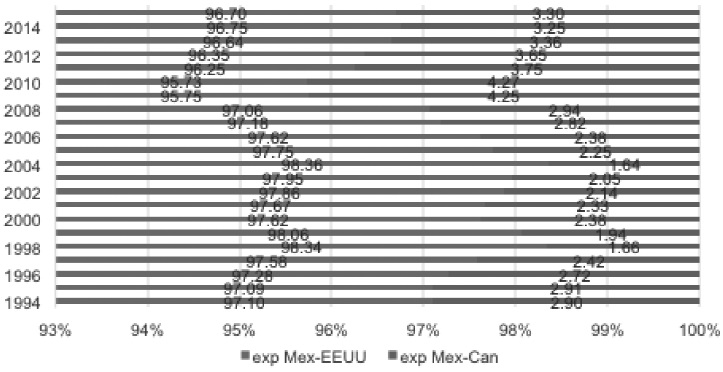
Between 1994 and 2015, exports from Mexico to the United States averaged 97.21%, well above those to Canada (2.79%) (Figure 1).
Imports by Mexico had the same behavior; of the total imports made from North America, 95% come from the United States. However, imports from Canada increased over time, going from 2.87% in 1994 to 6.08% in 2009 (Figure 2); at the same time, imports from the United States tended to decrease, from 97.13% to 93.92%.
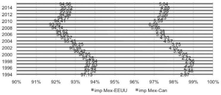
Source: Own elaboration with data from the IMF.
Figure 2 Imports received by Mexico from Canada and the US.
As can be observed, one of the consequences of NAFTA was the great geographical concentration of trade flows within this trade bloc. According to the International Monetary Fund (IMF), in 2012 more than 80% of the total foreign trade of the trading partners was concentrated in the North American bloc. The United States became the regional articulating axis, and Mexico and Canada increased their commercial and economic dependence on this country.
The geographical distance between the three countries is considered to have been a variable that favored the concentration of trade flows around the United States. In the article we use this variable to estimate our gravitational models and construct the “instrumental variables”.
Bilateral trade intensity of imports and exports3 between the three countries
Between 1994 and 2014, the trade flows (exports and imports) of the three partners maintained the same trends, and the only differences were in the magnitudes exported from each country (Figure 3):
Exports from Canada to Mexico and the United States have the highest intensity index. They are followed by those from the United States to Mexico and Canada; and finally, those from Mexico to Canada and the United States. Thus, the indices of Mexico and the United States were lower than those of Canada, so that exports from this country increased within this trade bloc, and increased trade interdependence between them.
The United States is the main recipient of Mexican and Canadian exports.
Mexican exports have the same trend as those of the United States and Canada but remain at a much lower level; that is, Mexico is the country that exports the least under NAFTA and is the largest recipient of U.S. and Canadian exports.
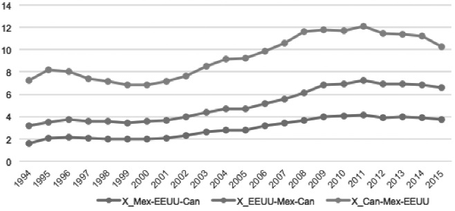
Source: Data from the Un-Comtrade, own calculations for the index.
Figure 3 Bilateral Export Intensity Index in NAFTA.
With regard to the intensity of imports from the region, Figure 4 shows that:
The United States is the largest importer in the region and had a six-point gap in the import intensity index with respect to Canada between 2007 and 2012.
The rate of bilateral imports from Mexico and Canada was lower than that of the United States and the rate of imports from Canada was higher than that of Mexican imports.
Mexico’s intensity index was the lowest, and the flow of imports between the United States and Canada was more intense; therefore, the Mexican market was not very relevant for the United States and Canada.
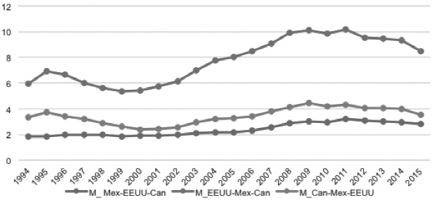
Source: Data from the Un-Comtrade. Own calculations for the index.
Figure 4 Bilateral Import Intensity Index in NAFTA
On the other hand, it should be noted that China coincidentally appeared on the NAFTA scene as a fourth player following the recession of 2000-2001. From 2001 onwards, China joined world trade by joining the World Trade Organization (WTO) and, although it was not a member of the Treaty, it almost immediately joined the economic dynamic of the North American trade bloc. China has been a de facto participant, predominantly in the trade exchanges of the three nations, so it became the main partner of the U.S. economy, displacing Mexico to third place in 2003, and Canada to second place in 2009. Regarding Mexico and Canada, China became the second supplier after the United States (López Arévalo, J. et al., 2014). However, in the case of Canada, this does not represent a weakening of its commercial position vis-à-vis the United States, because they are not competitive markets, since Canada is basically a supplier of natural and energy resources (Montero Delia and Enrique Pino, 2014). But in the case of Mexico, the situation is different because “competition with Chinese manufactures in the U.S. market not only faces low labor costs, quality and price, but the technological content and trade structure also falls on similar manufactures” (Montero Delia, Enrique Pino, 2014: pp.163). However, despite this, according to López Arévalo, J. (2014) Mexico maintained certain advantages over China, having increased vertical and horizontal intra-industry trade, while China has basically developed horizontal intra-industry trade.
Review of the literature
Theoretical review
Since the 1950s, neoclassical economic theory has studied the factors that explain the economic growth of countries, such as the accumulation of physical capital, exogenous technical progress and innovations that improve total factor productivity. According to this theory, productivity has a fundamental explanatory role in the growth phenomenon. After the Second World War, the world economy maintained very high economic growth rates associated with increased investment and the expansion of world trade. In the 1990s, interest in economic growth measured by per capita income appeared again; however, this time it is a question of explaining growth by the interdependence between countries with different levels of development, international trade, the accumulation of human capital, and endogenous technical progress.
The theory of exogenous growth assumes that economic growth is limited by the existence of decreasing returns on capital. Thus, in a closed economy, capital accumulation, by raising per capita income and increasing capital stock, reduces production and diminishes the incentive to continue accumulation. However, the argument changes in the context of a small open economy, because the specialization derived from international trade counteracts the negative effects of declining returns to capital on growth; this type of economy, which takes international prices, maintains the terms of trade constant and is not sensitive to the size of the capital stock. In this case, the terms of trade remain constant regardless of whether the country grows or not. If the economy specializes only in a labor-intensive good, capital accumulation will increase the production of this good, and the country will be able to exchange it, at fixed prices, for the goods produced by the world market. However, the fall in purchasing power in the international markets of the economy and declining returns on capital will cause a fall in per capita income.
According to Schott (2003), if this open economy diversifies and produces “n” different final goods, with different capital intensities, accumulation modifies specialization by orienting it towards sectors with greater capital intensity. And marginal productivity of capital declines as a result of the transition of this low capital-intensive economy to a higher capital intensity. Thus, the process of capital accumulation diversifies the economy. According to Ventura (1997), this explains why small economies grow faster than large ones, as they are able to offset the adverse effects of declining returns on a capital scale through international trade. Young (1992) considers that the structural transformations of Hong Kong and Singapore illustrate the validity of this theory. On the other hand, Griffin and French-Davis (1964) argue that international trade leads to an equalization of factor prices and per capita income among participating countries. In this manner, one country may grow at the expense of another provided that the price-to-income elasticities of the exports of the countries involved in trade are low. Finally, it should be noted that all the literature in this field of study is based on the theory of comparative costs.
Since the 1980s, empirical evidence has shown the existence of non-convergence of per capita income between poor and rich countries in the world economy. To explain this new reality, the theory of endogenous growth emerged, which tried to relax the assumption of declining returns by introducing human capital. Although this theory relaxed the hypothesis of diminishing returns on capital, it maintained the analytical foundations of the neoclassical theory.
“The explanation for the ‘new’ theory of growth is that there are forces of action that prevent the marginal product of capital from decreasing (and the capital-to-product ratio from increasing) as investment grows and (...) countries become richer” (Thirlwall, 2003:65). The theory of endogenous growth assumes the existence of a direct relationship between the capitallabor ratio and the productivity of capital. Thus, as investment increases the capital-to-product ratio, per capita output increases and each country grows at the same per capita rate.
The theory of endogenous growth considers that the effects of knowledge diffusion flows between countries explain to a large extent the relationship between international trade and per capita income growth. The endogenous growth theory models used the “learning-by-doing” concept of Arrow (1962) to explain how to counteract the trend towards diminishing returns on capital accumulation. These models assume that automatic knowledge generation is a byproduct of investment and that it has a positive cumulative effect on production and total industry productivity. So that any company, by increasing its physical capital, simultaneously learns to produce more efficiently; this process is called “learning by doing”. Thus, the higher the level of accumulation in a given industry, the more important the stock of knowledge that exists in it and the more productive are its inputs.
Thus, in the context of international trade, the extension of the international effects of the diffusion of “learning by doing” affects the structure of international trade and the growth of the per capita income of the countries. Therefore, this “learning by doing” may take place at the national or international level.
According to Grossman and Helpman (1995), in the long-term, the productivity growth of a country depends on the structure of its demand and the initial stock of knowledge. From the perspective of these authors, in the case of a country that produces two highly substitutable goods, it will specialize in only one of them in the long-term, and this is due to the differences in the initial conditions of the knowledge stock in each of the sectors. If the relative stock of initial knowledge is high in one sector, it tends to overflow in favor of a specific sector, which in the long run expands and dominates the entire economy. On the other hand, if the other sector has a low initial learning speed, the opposite evolution occurs. So, in this economy, the long-term growth rate of per capita income will depend on the initial conditions of the state of knowledge and learning, that is, on the initial conditions of the stock level of knowledge and the speed of learning, which can be high or low.
However, if two economies with a different specialization profile exchange their products, their growth will depend on international trade generating interaction and ‘learning by doing’, producing a positive flow of knowledge between them. In the event that both countries have the same initial stock of knowledge, their specialization profile would be determined by comparative advantages and their intrinsic level of productivity. In this case, this interdependence can generate various results since a country may specialize in a sector with low growth potential, or in a high potential sector. On the other hand, if the “learning by doing” process is only national in scope, patterns of specialization become entrenched and strengthened over time. Thus, each country becomes more productive in sectors that have comparative advantages. In this case we would have to assume that per capita income growth rates do not necessarily converge, so that in these conditions international trade does not lead to convergence of the growth rate, nor does it lead to the rapid growth of countries.
On the other hand, there are a number of models where investment in research and development (R&D) affects per capita income growth. According to these models, R&D has two channels through which it can affect growth: through the impact on the range of products available, and through the impact on the stock of knowledge available for R&D investment. In the international context, 95% of R&D is carried out in developed countries, and if the results of R&D are confined to these countries, it becomes a factor contributing to the disparity in the living standards of the world population.
According to Grossman and Helpman (1991), endogenous growth theory does not predict a one-way causal relationship between international trade and productivity growth. Rather, they consider that the relationship between the two is not defined, as investment in R&D may encourage or discourage growth in per capita income, whatever the case may be. Romer (1986) points out that free trade will be more beneficial for a country with more human capital than for one with only a large population. Frankel and Romer (1999) study the relationship between international trade and per capita income applying the geographical approach, and develop an empirical methodology, based on the construction of instrumental variables, to study the interrelationships between the two.
Empirical contributions
There are many empirical studies on the relationship between exports and economic development. Tyler (1981) uses a cross-sectional model to prove that the association between exports and imports is positive for 55 countries. Ram (1985) uses a production function to demonstrate the export drive on economic development in developing countries; the results of their study corroborate the fact that export performance is important for promoting economic development. Mbaka and Paul (1989) analyze the relationship between exports and economic development from a production point of view. These authors find that there is a significant effect on middle-income countries, while the effect is not relevant in low-income countries. Starting in 1985, according to Anoruo and Ahmad (2000), they changed the usual empirical approaches, as researchers began to use the causality test to determine the direction of causality between exports and economic development. The first causality studies were conducted by Jung and Marshall (1985) and Chow (1987). Jung and Marshall used the causality test developed by Granger (1969), the result of which opens the discussion around the hypothesis of export promotion. Dodaro (1993) suggests that this causality test offers weak support for strengthening the thesis that trade is the engine of development. Chow (1987) analyzes the causal relationship between economic development and exports for eight countries that fall into the category of newly industrialized countries (NIC). Using the Sim causality test, it is revealed that in most NICs there is a strong dual causality directionality between exports and industrial economic development.
Concerning the empirical work done on intra-NAFTA trade, we find that Thornton (1996) conducted a cointegration analysis (using the Engel-Granger methodology) for Mexico for the period of 1985 to 1992; the author finds that there is a unidirectional causality of exports to per capita income. For their part, Cheng and Chu (1996) apply the Phillips-Perron unitary root test and the Engel-Granger method of integration for the United States and find a two-way causality between per capita income and exports (Donoso and Martín, 2002). According to Anoruo and Ahmad (2000) and Donoso and Martin (2002), these differences in results may be due to several factors such as differences in procedures, specified delay structures, or data filtering techniques.
Calderón and Plascencia (2007) studied the relationship between growth and economic openness in the three NAFTA countries, used a time series analysis of quarterly data for the 1984:1 to 2003:2 period, and applied the Engel-Granger co-integration method to determine the existence of long-term relationships between growth and economic openness for each of the countries. They concluded that Mexico was the only country where a long-term relationship exists.
Cyrus (2002) used a gravitational model to demonstrate a positive relationship between trade and income. Furthermore, it considers that the size of countries and the formation of trade blocs are important in bilateral trade, and that non-formal blocs have the greatest impact on this type of trade.
On the other hand, Josheski and Fotov (2013) also used the gravitational model with control variables such as transport costs, trade between neighbors and the existence of coastlines. These authors apply three models, ordinary least squares, instrumental variables and Poisson, to analyze the relationship between trade and the creation (diffusion) of technology. In addition, they show that there is a high dependency between levels of technology exports and imports and bilateral trade flows.
After analyzing the current scope of empirical literature, despite its advances, we can conclude that it does not precisely explain the nature of the relationship between international trade and development. Most of the studies available do not establish an exact directionality in their estimates of the relationship between exports and economic development. So, while in some econometric analyses a one-way relationship is established, in others a two-way relationship is found.
Model methodology
In this article we returned to the empirical methodology developed by Frankel and Romer (1999), using instrumental variables to study the relationship between international trade and the economic development (GDP per capita) of the NAFTA partners. Based on this methodology, we first estimated a cross-country regression of the relationship of per capita income and GDP of the countries, then applied a gravitational model of trade with geographical factors to explain bilateral trade. In the gravitational equation we only use geographical variables (size of the country, the distance between them, if they share a border or if they have coastlines) (Sánchez, 2010: 58). Geographical factors have a positive relationship on the bilateral trade of the region, the reduction of transport costs favors production, raises GDP levels, and positively affects the level of per capita income. All the variables used, except the dummies, were transformed into logarithms to interpret the results in terms of elasticities (Sánchez, 2010: 59).
Following the methodology of Frankel and Romer (1999) to measure the impact of bilateral trade on per capita income, we construct, in the first place, the Instrumental Variable4 (IV) from the variables per capita income5, size of the three countries6; proximity between countries7; international trade8, and the dummy variables9.
For this, we used a three-equation model10. The first one explains the average income (Yi, per capita income) of each of the three countries, according to their respective interaction (Ti) and the internal variations of each of them (whiting-country, Wi), and εi11:
The second explains bilateral trade in terms of the proximity of the three countries Pi; and δi of other factors
Where: Ti: is the total trade of the countries12 divided by the GDP. Ti is the sum of the bilateral trade of country (i) with each of the other countries of the sample13.
The third equation focuses on within-country trade, which is the function for the size of the country (Si) and of other factors14. (Sánchez, 2010:60).
To create the instrumental variable, equations (2) and (3) are replaced in equation (1)15 and the following relation is obtained:
Equation (4) is estimated using the variables: geographical proximity (Pi), size of each country (Si,), constant, and instruments16. From it we obtain the parameter (β) which is the elasticity that measures the impact of bilateral trade on income; also (γλ), which is the elasticity of the impact of the size of the country on income. It should be noted that the components of coefficient (γλ) are not identified separately, it is not possible to obtain only the estimate of (γ) of within-country trade on income, just as it is not possible to obtain only (λ). So, if (λ) is positive it implies that the larger a country is, the more it will have a greater within-country trade and the sign of (γ) will be of the same sign as (γλ). Thus, although these elasticities cannot be directly obtained separately, the value of their sign can be obtained (Sánchez, 2010)17.
If Pi and Si are negatively correlated, it means that the larger a country is, the more dispersed its market is and the further away it is from other countries. So, if you take the country size (Si) as a control variable in (4), (Pi) would be negatively correlated with the residual and you would not have a valid instrument; which indicates that small countries increase their participation in bilateral trade with other countries when within-country trade is lower. If not taken in (4) to (Ti) as the control variable, then (Si) is negatively related to the residual and cannot be estimated. Therefore, the impacts of both international trade and the size of the country must be examined (Sánchez, 2010)18.
As a second step, the bilateral trade equation is constructed using the gravitational model19 of bilateral trade, which shows how trade between countries (Tij) is negatively related to the distance between them (Dij,2120) and positively related to their sizes (Si and Sj) (size of the income per capita of the two countries) (Sánchez, 2010).
The specification of the bilateral trade equation would be21:
Geographic information is aggregated to identify the geographic influence on global trade that includes measures of magnitude (log population (lnN) and log area (lnA)) and dummy variables. The latter explain whether or not the country has coastlines (L) or whether they share borders (B). The new equation to be estimated is as follows22:
The third step in the methodology by Frankel and Romer (1999) is the construction of the virtual variable that measures aggregate trade and helps finding the implications of estimating the geographic component of countries on total trade. To do this, the adjusted values of the bilateral trade equation are added together and equation (6) (Sánchez, 2010) is simplified as follows:
Where: is the coefficient vector in (6) and (α0, α1, ..., α13); (Xij) is the vector on the right side of the variables (1, lnDij, ..., Bij (Li+Lj))
To complete the equation, the proportion of trade constructed for all countries was included, which is derived from the estimation of the geographic component of country (i) as a share of global trade:
According to equation (8), the estimate of the geographical component of regional trade (i) is the sum of the estimates of the geographical components of the bilateral trade23 of the member countries. To make the calculation, it is necessary to know the data on the populations of the countries and their geographical characteristics (Sánchez, 2010).
Finally, the effects of trade on per capita income are estimated using the Instrumental Variables (IV). The dependent variable is the logarithm of per capita income (Sánchez, 2010), the estimated period is from 1994 to 2015.
The difference between equation (9) and equation (1) is that the latter includes two magnitudes, population (N) and area (A), which are the geographical factors used in the construction of the instrument to support the analysis. (Sánchez, 2010).
Empirical Results
Bilateral Trade
The bilateral trade equation was estimated using data from the Census Bureau, IMF and Penn World Table 9.0; the units of measure are millions of dollars. The distance is taken from Haveman Jon and calculated as an orthodromic distance from Mexico City, Ottawa, and Washington. The population was taken from the Penn World Table. The size of the countries is measured in square kilometers. Two dummy variables were constructed between the countries where there is a common border, and which have coastlines. Mexico and the U.S. have a common border, so the value of one is assigned; while there is no common border between Mexico and Canada, so the value of zero is assigned. The second dummy variable is the existence of coastlines and given that the three countries have them, they are assigned the value of one (Sánchez, 2010: 67).
We use annual data to study the period of 1994 to 2015. The bilateral trade equation between NAFTA members was estimated using a panel model-estimated by ordinary least squares (OLS), fixed effects (FEs), random effects (REs) and generalized least squares (GLS)-the results are shown in Table 1 summarizing the four tests applied to the estimate. It shows the values of the estimated coefficients, the standard errors of the variables, and the p-value of the test t, which show the individual significance of the variables used.
Table 1 Bilateral trade in the NAFTA
| 1.OLS | 2.GLS | 3. Fixed Effects | 4.Random Effects | |||||
|---|---|---|---|---|---|---|---|---|
| A.Variable | B.Interacción | A.Variable | B.Interacción | A.Variable | B.Interacción | A.Variable | B.Interacción | |
| Constant | -76.91601 | -76.91601 | -35.36882 | -75.23937 | ||||
| (4.083765) | (3.958081) | (10.70586) | (4.43627) | |||||
| p-value 0.000 |
p-value 0.000 |
p-value 0.001 |
p-value 0.000 |
|||||
| -0.391178 | -1.2871 | -0.3911784 | -1.2871 | -0.425557 | -1.217691 | -0.392565 | -1.284299 | |
| Ln distance | (0.03662) | (0.052289) | (0.035499) | (0.0506799) | (0.033901) | (0.049835) | (0.03488) | (0.049868) |
| p-value 0.000 |
p-value 0.000 |
p-value 0.000 |
p-value 0.000 |
p-value 0.000 |
p-value 0.000 |
p-value 0.000 |
p-value 0.000 |
|
| 5.851389 | -1.675618 | 5.851389 | -1.675618 | 1.577026 | -1.675618 | 5.678897 | -1.675618 | |
| Ln population | (0.412943) | (0.5839904) | (0.400234) | (0.5660172) | (1.099223) | (0.523991) | (0.450420) | (0.555519) |
| p-value 0.000 |
p-value 0.005 |
p-value 0.000 |
p-value 0.003 |
p-value 0.154 |
p-value 0.002 |
p-value 0.000 |
p-value 0.000 |
|
| -2.114018 | -0.6127993 | -2.114018 | -0.6127993 | 0.4990972 | -0.577891 | -2.008565 | -0.6113906 | |
| Ln size | (0.255124) | (0.363209) | (0.247272) | (0.3520307) | (0.672817) | (0.32600) | (0.27758) | (0.345506) |
| p-value 0.000 |
p-value 0.094 |
p-value 0.000 |
p-value 0.082 |
p-value 0.460 |
p-value 0.079 |
p-value 0.000 |
p-value 0.057 |
|
| 26.93065 | 26.93065 | 26.3922 | 26.90893 | |||||
| Slit_ij | (2.852638) | (2.764844) | (2.5628) | (2.713705) | ||||
| p-value 0.000 |
p-value 0.000 |
p-value 0.000 |
p-value 0.000 |
|||||
| Sample size | 132 | 132 | 132 | 132 | ||||
| R2 | 0.9879 | |||||||
| Adjusted R | 0.9872 | |||||||
| root MSE | 0.19861 | |||||||
| prob. F | 0.0000 | 0.0000 | ||||||
| prob. chi | 0.0000 | 0.0000 | ||||||
| R sq within | 0.9916 | 0.9904 | ||||||
| R sq between | 0.9185 | 0.9185 | ||||||
| R sq overall | 0.9669 | 0.9878 | ||||||
Satandard errors between parenthesis. Level of significance at (5%)
The columns represent the results of the estimates made by means of Ordinary Least Squares (1.OLS), Generalized Least Squares (2.GLS), 3.Fixed Effects, and 4.Random Effects, respectively (Sánchez, 2010: 67-68).
Column A records the results of the estimation of per capita income from the logarithm of the simple variables (ldist, lpob, ltam, and litij); and column B shows the results of the interactions formed by variables composed between the border variable and the rest (borderto-population, border-to-distance, border-to-size), and the dummy border-to-coastline variable.
The results are the following:
The distance variable has a negative sign and its elasticity coefficient is significant, implying that there is an inverse relationship between bilateral trade and distance; and it is confirmed that the greater the distance between the trade centers of each country, the greater the cost of transporting goods and the lower the bilateral trade will be.
The size of the country has a negative sign, implying that a country with a larger territory will have a less homogeneous domestic consumption market and bilateral trade will have a higher cost to conserve local consumption.
The population has a positive sign, indicating that the country with the largest number of inhabitants tends to be a larger consumer market and contributes to the increase in bilateral trade.
The second column corresponds to the results of the interactions between the border variable and the other variables; the results of these interactions are also consistent with expectations:
The signs of the interactions between border-distance, border-size and border-population are negative, as are the results in column A; however, for the non-coastline variable they are positive, which supports the idea that a country that has coastlines and shares borders contributes positively to the increase in bilateral trade. (Sánchez, 2010)
From the results of Hausman’s test24 the specification is chosen by random effects. The estimator derived from this specification converges to the ordinary least squares estimator, because the unobservable effect of the error term is of little relevance since its variance may be small. This indicates that there is homogeneity in the behavior of the variables. (Sánchez, 2010).
According to Hausman’s test, the null hypothesis is not rejected, so there is no systematic difference between the coefficients and it is decided to choose the random effects model that has the efficient estimator.
| Hausman’s test | ||||
|---|---|---|---|---|
| Coefficients | ||||
| (b) Consistent | (B) Eficient | (b-B) Difference | Sqrt(V_b-V_B)) S.E. | |
| ltam | 0.4990972 | -2.008565 | 2.507662 | 0.61288 |
| lpob_calc | 1.577026 | 5.678897 | -4.101871 | 1.002703 |
| ldist | -0.4255578 | -0.3925657 | -0.0329921 | - |
| f_Ipob_calc | -1.675618 | -1.675618 | -6.95e.10 | - |
| f_Itam | -0.578913 | -0.6113906 | 0.0334993 | - |
| f_Idist | -1.217691 | -1.284299 | 0.0666071 | - |
| f_litij | 26.39229 | 26.90893 | -0.5166366 | - |
| b = consistent under Ho and Ha; obtained from xtreg | ||||
| B = inconsistent under Ha, efficient under H0; obtained from xtreg | ||||
| Test: H0: difference in coefficients not systematic | ||||
| chi2(7) = (b-B)’[V_b-V_B)ˆ(-1)](b-B) | ||||
| = 16.69 | ||||
| Prob>chi2 = 0.0202 | ||||
In the table above, the results of both estimates are reported for comparison and analysis purposes.
Built Aggregate Trade (virtual variable)
From equation (6), the adjusted total trade equation is constructed, which we will call virtual. With this, the aggregate trade for each country per year is calculated. From there, we can move on to the next step, which is to estimate the impact of aggregate trade on per capita income (Sánchez, 2010:71).
First, equation (6) is adjusted as follows:
In 6A, the dependent variable is the logarithm of bilateral trade (obtained in the previous stage), and the independent variables are the natural logarithm of the distance between two countries, the natural logarithm of the population, the natural logarithm of the area, the interaction between the border and the natural logarithm of the distance, border and the natural logarithm of the population, the border and the natural logarithm of the magnitude and, finally, the border with the coastlines25.
Aggregate equation (7) is solved
Where:
α’ is the row vector of the coefficients, and (Xij) is the matrix of the temporary variables.
This is:
And finally, the aggregate trade variable is obtained by incorporating the geographical component of the countries in global trade:
Thus, the aggregate trade built from equation (8) is a function of population, country size, and income per worker. To estimate the effects of bilateral trade on the per capita income of each country, we use the bilateral trade data from the Penn Table (Sánchez, 2010:72).
Evaluation of the quality of the Instrument Variable
To evaluate the quality of the built instrument variable, we studied the relationship between the aggregate trade built and the current trade (trade openness index) in each country. And we compare the three models estimated by random effects; the first one defines only the relationship between current trade and aggregate trade built; the second econometric model omits constructed aggregate trade and takes into account size and population; and the last one is a more complete model, which considers geographical variables of size and population, and aggregate trade built (Sánchez, 2010). The results are shown in Table 2.
Table 2 Relation between Real Trade and Aggregate Trade Built.
| Variable | Model 1 | Model 2 | Model 3 |
|---|---|---|---|
| Constant | 15.26971 (1.347871) | -534.0274 | -500.6002 |
| P-value 0.000 | (186.1594) | (156.5931) | |
| P-value 0.004 | P-value 0.001 | ||
| Aggregate Trade Built | 0.0075511 | 0.0054642 | |
| (0.0824017) | (0.0007404) | ||
| P-value 0.000 | P-value 0.000 | ||
| Ln population | 33.34278 | 34.56165 | |
| (19.24573) | (16.18315) | ||
| P-value 0.083 | P value 0.030 | ||
| Ln tam | -5.49012 | -9.352944 | |
| (11.93739) | (10.0509) | ||
| P-value 0.646 | P-value 0-352 | ||
| Sampled size | 132 | 132 | 132 |
| R2 within | 0.3663 | 0.4357 | 0.6097 |
| R2 between | 0.2890 | 0.7786 | 0.7086 |
| R2 overall | 0.3520 | 0.4446 | 0.6103 |
| Prob. Chi2 | 0.0000 | 0.0000 | 0.0000 |
Standard errors between parentheses. Level of significance at (5%).
The relationship between Real Trade and Aggregate Trade Built is shown in Table 2. In the three models that were estimated, the relationship between real trade (dependent variable) and independent trade (geographical) is shown. Models one and three include the aggregate trade built variable, which is significant in both estimates. Model three, which is the most complete, as it includes the geographical variables of population and size, has the most significant estimators. In this model, the relationship between the real trade Τ and the aggregate trade built is significant, the population is also significant, and the size is not significant. The relationship between the variables varies from country to country and is positive. The correlation between real trade and aggregate trade built is significant (Sánchez, 2010).
Effects of bilateral trade on per capita income in the NAFTA region
To capture the effects of bilateral trade on the per capita income of the three countries, we used the instrument constructed to estimate relationship (9A). This instrument is inserted into equation (9) and the following equation is obtained (Sánchez, 2010)26:
Where the dependent variable is the natural logarithm of per capita income27 (lnYi); (Ti) is the real trade (trade openness index of each country); (Ni) and (Ai) are the population and area, respectively. Regression is estimated with random effects (RE) and instrumental variables (IV) based on the aggregate trade constructed. . The results are shown in Table 3.
Table 3 Effect of Trade on Income.
| (1)(9) | (2)(9A) | |
|---|---|---|
| Estimation | RE | VI |
| Constant | -78.6984 | -83.14959 |
| (5.39277) | (6.010463) | |
| p-value 0.000 | p-value 0.000 | |
| Real Trade (Ti) | -0.0716245 | |
| (0.0024729) | ||
| p-value 0.000 | ||
| Trade Built | -0.0799597 | |
| (0.0047228) | ||
| p-value 0.000 | ||
| Ln population (Ni) | 7.096669 | 7.374589 |
| (0.5467986) | (0.5855961) | |
| p-value 0.000 | p-value 0.000 | |
| Ln tam (Ai) | -2.639089 | -2.68485 |
| (0.335555) | (0.3508033) | |
| p-value 0.000 | p-value 0.000 | |
| Sample size | 132 | 132 |
| R2 within | 0.9262 | 0.9278 |
| R2 between | 0.2717 | 0.1776 |
| R2 overall | 0.9001 | 0.8981 |
| Prob. Chi2 | 0.0000 | 0.0000 |
Standard errors between parentheses.
Level of significance at (5%).
Column 1 shows the results of the estimation of equation (9) by random effects (RE), and the second column is the estimation of equation (9A) through the instrumental variable (IV) represented by the constructed trade. The results of these estimates show that there is no evidence to indicate a positive relationship between increased trade and increased income, and that this leads to long-term economic growth. Random-effects results show that real trade and per capita income have a negative relationship (Sánchez, 2010: 77), indicating that by increasing trade by 1%, the per capita income of the region decreases by 7.1%. The relationship between the size of the country and the dependent variable is negative, which implies that the larger country will have a lower increase in per capita income.
In reference to the estimation with the instrumental variable (IV), the results with respect to population and size are the same as with random effects. As regards the aggregate trade built, it has the same negative sign, but it is not significant, showing the existence of an inverse relationship between the increase in trade and per capita income. There is a difference between the estimates with (RE) and with (IV), the first one being determined by the partial association between per capita income and bilateral trade, and the estimate with (IV) being determined by the partial association between income and the trade component that correlates with the instrument.
Conclusions
The results of the article are important because they show that there is a negative relationship between trade and per capita income in the NAFTA region. This is corroborated both in the estimation of equation (9), which integrates real trade, and in the estimation of equation (9A), which integrates the trade built variable. This would indicate that as intra-NAFTA trade expands in the region, the standard of living of the population is declining. This model takes up the existing diversity in the region in geographical and economic terms where three countries with different levels of development coexist. This would explain why openness did not favor per capita growth in the region. Since, according to endogenous growth models, there were no technological spillovers for the NAFTA countries, neither on the side of trade in final products nor on the side of trade in specialized inputs.
In addition, we conclude that the country with the largest population and the largest area of land is the one more benefited from NAFTA, so this agreement tended to favor the country that meets these two conditions, that is, the United States. And, on the other hand, in the case of the Mexican economy, which has the smallest population and the smallest territory, it is the most affected by this negative relationship. Mexico underwent profound structural changes that affected its accumulation scheme and went into a state of chronic stagnation of underemployment.
REFERENCES
Arrow, K. (1962). “The economics implications of learning by doing”, Review of Economic Studies, núm. 29, pp. 150-173. https://doi.org/10.2307/2295952 [ Links ]
Banco Mundial (S/F) disponible en: http://www.bancomundial.org/ [ Links ]
Calderón, C. & Plascencia, I. (2007). “Does Economic Opening in Mexico Promote Economic Growth?” in Studies of Sweden and Mexico: Economics, Finance, Trade and Environment. Ed. by Ignacio Perrotini Hernández and Fadi Zaher. [ Links ]
Calderón, C. & Hernández, L. (2011), “El TLCAN una Forma de Integración Dualista: Comercio Externo e Inversión Extranjera Directa”, Estudios Sociales, vol.37, pp. 91-118. [ Links ]
Cheng, B. & Chu, Q. (1996). “U.S. Exports and Economic Growth Causality”, Atlantic Economic Journal, núm. 24. https://doi.org/10.1007/bf02298512 [ Links ]
Chow, G. (1987). “Money and price level determination in China”, Journal of Comparative Economics, volume 11, No. 3, pp. 319-333. https://doi.org/10.1016/0147-5967(87)90058-8 [ Links ]
Cyrus, T. (2002). “Income in the Gravity Model of Bilateral Trade: Does Endogeneity Matter?”, The International Trade Journal, volume XVI, núm. 2. https://doi.org/10.1080/08853900252901404 [ Links ]
Dodaro, S. (1993). “Exports and growth: A reconsideration of causality”, The Journal of Developing Areas, vol.27, núm. 2, pp. 227-244. [ Links ]
Donoso y Martin (2009). “Exportaciones y Crecimiento Económico: estudios empíricos” ICEI, WP05/09. Disponible en: https://dialnet.unirioja.es/servlet/articulo?codigo=3048896 [ Links ]
Fondo Monetario Internacional (FMI), Estadísticas de Comercio Internacional. Disponible en: Disponible en: http://www.imf.org/external/index.htm . Consultado el 08/06/2016. [ Links ]
Frankel, J. & Romer, D. (1999). “Does Trade Cause Growth?” American Economic Review, vol. 89, Issue 3, pp. 379-399. https://doi.org/10.1257/aer.89.3.379 [ Links ]
Granger, C. (1969). “Investigating Causal Relations by Econometric Models and Cross-spectral Methods”, Econometrica, vol. 37, núm. 3. pp. 424-438. https://doi.org/10.2307/1912791 [ Links ]
Griffin, K. & French-Davis, R. (1964). “Comercio internacional y modelos de crecimiento a largo plazo”, Desarrollo Económico, vol. 3, núm. 4, pp.585-605. https://doi.org/10.2307/3465792 [ Links ]
Grossman, G. & Helpman, E. (1995). Technology and trade in Gene M. Grossman y Kenneth Rogoff, eds. Handbook of international economics, vol. 3, Elsevier, Amsterdam. https://doi.org/10.1016/s1573-4404(05)80005-x [ Links ]
Grossman G. & Helpman, E. (1991). “Quality ladders in the theory of Growth”, Review of Economic Studies, núm. 58, pp. 43-61. https://doi.org/10.2307/2298044 [ Links ]
Grossman G. & Helpman, E. (1989). “Product Development and International Trade”, Journal of Political Economy, núm. 97, pp.1261-1283. https://doi.org/10.3386/w2540 [ Links ]
Hausman, J. (1978). “Specification tests in econometrics”, Econometrica, vol. 46, núm. 6. https://doiorg/10.2307/1913827 [ Links ]
Haveman’s, J. (S/N) “International Trade data” Disponible en http://www.macalester.edu/research/economics/PAGE/HAVEMAN/Trade.Resources/TradeData.html [ Links ]
Hufbauer, G. & Schott, J. (2005). NAFTA Revisited: Achievements and Challenges, Institute for International Economics. ISBN-13:978-0881323344 [ Links ]
Instituto Nacional de Estadística Geográfica e Informática (INEGI). Disponible en: http://www.inegi.org.mx/ [ Links ]
Josheski, D. & Fotov, R. (2013). “Gravity Modeling: International Trade and R y D”, University Goce Delcev-Stip. Disponible en: http://mpra.ub.uni-muenchen.de/45550/. núm. 45550 [ Links ]
Jung, W. & Marshall, P. (1985). “Exports, Growth and Causality in Developing Countries”, Journal of Development Economics, vol. 18, issue 1. https://doi.org/10.1016/0304-3878(85)90002-1 [ Links ]
López Arévalo, J., A., Rodil O., & Valdéz Gastelum, S. (2014). la irrupcion de China en el TLCAN: efectos sobre el comercio intra-industrial. Economia Unam, 11 (31), 84-113. https://doi.org/10.1016/s1665-952x(14)70446-3 [ Links ]
Mbaka, J. & Paul C. (1989). “Political Instability in Africa: A Rent Seeking Approach”, Public Choice, vol. 63, pp. 63-72. https://doi.org/10.1007/bf00223272 [ Links ]
Montero, D. & Pino, E. (2014). Presente y futuro de las relaciones comérciales de Canadá y Estados Unidos frente a los nuevos desafíos, Norteamérica, año 9, número 2. https://doi.org/10.20999/nam.2014.b006 [ Links ]
Monthly Statistics of International Trade, OECD, http://www.oecd.org/ [ Links ]
Moreno-Brid, J.C.& Ros, J. (2010). Desarrollo y crecimiento en la economía mexicana, México, Fondo de Cultura Económica. [ Links ]
Ram, R. (1985). “Exports and Economic growth in Developing Countries: Evidence from Time Series and Cross-Section Data”, Economic Development and Cultural Change, vol.36, pp.51-72. https://doi.org/10.1086/451636 [ Links ]
Romer, P. (1986). “Increasing returns and long run growth”, Journal of Political Economy, No. 94 pp.1002-1037. https://doi.org/10.1086/261420 [ Links ]
Sánchez, S. (2010). Crecimiento económico y comercio exterior de México en el marco del Tratado de Libre Comercio con América del Norte, TLCAN, 1994-2008. Tesis de Maestría, Maestría Economía Aplicada. El Colegio de la Frontera Norte, México. [ Links ]
Schott, P. (2003). “One size fits all? Heckscher-Ohlin specialization in global production”, American Economic Review, núm. 93, pp. 686-709. https://doi.org/10.1257/000282803322157043 [ Links ]
Thirlwall, A. (2003). La naturaleza del crecimiento económico, un marco alternativo para comprender el desempeño de las naciones. Fondo de Cultura Económica. México. [ Links ]
Thornton, J. (1996). “Cointegration, causality and export-led growth in Mexico, 1895-1992,” Economics Letters, Elsevier, vol. 50 (3), pp. 413-416. https://doi.org/10.1016/0165-1765(95)00780-6 [ Links ]
Tinbergen, J. (1962). Shaping the World Economy; Suggestions for an International Economic Policy. Books (Jan Tinbergen). Twentieth Century Fund, New York. Disponible en: http://hdl.handle.net/1765/16826 [ Links ]
Tyler, W. (1981). “Growth and export expansion in developing countries: Some empirical evidence”, Journal of Development Economics, vol. 9, issue 1, pp. 121-130. https://doi.org/10.1016/0304-3878(81)90007-9 [ Links ]
UnComtrade, WTO. Disponible en: Disponible en: https://www.wto.org/ . Consultado 17/05/2016 [ Links ]
Ventura, J. (1997). “Growth and interdependence”, Quarterly Journal of Economics, núm. 112, pp.57-84. https://doi.org/10.1162/003355397555127 [ Links ]
Young, A. (1992). “A tale of two cities: factor accumulation and technical change in Hong Kong and Singapore”, NBER Macroeconomic annual 1992, vol. 7, pp. 13-54 https://doi.org/10.2307/3584993 [ Links ]
2“Maquiladoras - Mexican firms with special legal status originally restricted to produce exclusively for export - are a closely watched feature of the Mexican economy. Common modus operandi that characterize maquiladoras: to import components, to add value (mainly through labor), and to export products (almost entirely to the United States)” Hufbaer and Schott (2005:48).
3The index is
4The tests with ordinary least squares (OLS), fixed effects (FE), random effects (RE) and generalized least squares (GLS) are performed, the true variance estimator is also applied using the White test and the Hausman contrast is performed to evaluate models with fixed effects and random effects.
5As a ratio between GDP at constant prices in millions of dollars and economically active population EAP.
9They indicate whether or not the country has coastlines (0 without coastlines and 1 with coastlines), and if they share a border (1 if they share a border and 0 without a common border). These dummy variables are an indicator of the effect of globalization and the trend towards higher real trade volumes. (Sánchez, 2010)
10Taking the model by Frankel and Romer (1999).
11Ԑi other income influences, this variable implies other channels through which trade afects income.
13Ti o Si1j (Tij/GDPi) Where Tij is the bilateral trade between country (i) and (j) (exports plus imports).
14The residuals of these three equations are correlated, but the geographic characteristics (Pi, Si) are not correlated with them. This is because proximity and size are not affected by income or other factors, such as government policies that do affect income. So, under the assumption that Pi and Si are not correlated with Ԑ, the data from Y, T, W, P, and S help us estimate equation (1). (Sánchez, 2010)
16The methodology used in Franker and Romer (1999) is used again.
17The methodology by Frankel and Romer (1999) is used again for the construction of a model with instrumental variables.
18Econometric conditions among the variables, following the methodology of instrumental variables used by Frankel and Romer (1999).
19One of the first studies to use the gravitational model was done by Tinbergen (1962), where it is established that the volume of trade between the two countries involved depends positively on their sizes, measured by their income levels; and negatively, on the transport costs involved between the distance from the economic centers, which is analogous to Isaac Newton’s theory. It was in 1966 with Linnemann that it is incorporated to the population as an approximate size of the countries (Tinbergen, 1962). (Sánchez, 2010)
20Orthogonal distance is the shortest path between two points on the earth’s surface, it is the arc of the maximum circle that joins them and is less than 180 degrees. (Sánchez, 2010)
21Methodology by Frankel and Romer (1999).
22Methodology by Frankel and Romer (1999).
23The expectation of
24Hausman’s test was proposed by Hausman in 1978; it is a chi-square test that determines whether the differences are systematic and significant between two estimates. It is mainly used to know whether an estimator is consistent and whether or not a variable is relevant.
25According to the methodology by Frankel and Romer (1999).
26According to the methodology by Frankel and Romer (1999).
Received: October 23, 2016; Accepted: February 07, 2017
 Este es un artículo publicado en acceso abierto bajo una licencia Creative Commons
