


Serviços Personalizados
Journal
Artigo
 texto em
  Inglês (pdf)
 Artigo em XML
 Referências do artigo
 Enviar este artigo por email
Indicadores
-
 Citado por SciELO
 -
 Acessos
Links relacionados
-
 Similares em
SciELO
Similares em
SciELO
Compartilhar

 Permalink
Contaduría y administración
versão impressa ISSN 0186-1042
Contad. Adm vol.63 no.4 Ciudad de México Out./Dez. 2018
https://doi.org/10.22201/fca.24488410e.2018.1204
Articles
The yield curve and its relation to economic activity in Mexico
1 Universidad Autónoma Metropolitana, México.
2 Universidad Anáhuac, México.
In this paper are analyzed the main components of the interest rate variation of debt instruments, issued by the Mexican Government, in the period 1978-2017. By means of an autoregressive vector, there is a relationship between these components and the variables: GDP gap, inflation rate and economic growth rate. Likewise, there is evidence of causality in the Granger sense, which establishes a bridge between the yield curve and economic activity in Mexico.
Keywords: Yield curve; fixed income; principal components; economic activity; Granger causality
JEL Classification: G19; C51; C52
En este trabajo se estudian los componentes principales de la variación de las tasas de interés de los instrumentos de deuda, emitidos por el Gobierno mexicano, en el periodo 1978-2017. Mediante un vector autorregresivo se encuentra una relación entre dichos componentes y las variables: brecha del PIB, tasa de inflación y tasa de crecimiento económico. Asimismo, se encuentra evidencia de causalidad en el sentido de Granger, lo que establece un puente entre la curva de rendimiento y la actividad económica en México.
Palabras clave: Curva de rendimiento; renta fija; componentes principales; actividad económica; causalidad en el sentido de Granger
Códigos JEL: G19; C51; C52
Introduction
The analysis of the interest rates of debt instruments in Mexico is a relevant exercise, as they are a monetary policy tool for the central bank, while homes and people base their decisions at the level and change of the interest rates. In this sense, this document seeks to contribute to the study of the temporary structure of interest rates1 for Mexico, since the fixed income market has become more and more sophisticated, due in part to the dynamics with international capital markets, as well as by the emergence of new financial instruments and the expansion-recession of the economy, such as the case of the of 2008-2009 financial crisis.
This work analyzes the principal components of the variation of the interest rates of debt instruments issued by the Mexican government during the period of 1978-2017. Subsequently, through Granger causality tests and a vector autoregression, a relation between said components and the variables was found: GDP gap, inflation rate, and economic growth rate. These results allow establishing a bridge between the yield curve and the economic activity in Mexico.
The document is organized as follows: first, the recent literature on this subject is reviewed; then, the second section reviews the principal component analysis and hypothesis tests; the third section presents the results of a vector autoregression; and finally, the conclusions are presented.
Review of the literature
A subject of great interest is the understanding on how the short segment of the temporary structure of interest rates relate to the long-term rates, and the underlying factors that could be affecting both the levels and variations of the rates, and how these rates are related to the real sector of the economy. In this context, the tools used were the principal component analysis and factor analysis, Martínez and Núñez (2012) and García (2011).
Concretely, as developed in Litterman and Scheinkman (1991) and subsequently in Knez, Litterman and Scheinkman (1996), using the principal component analysis, the common factors that affect the yields on the fixed income instruments in the United States are determined. To explain the variance of the yields it is necessary to distinguish or differentiate the systematic risk of the particular risk that affects each of the instruments. The common factors with which the above is explained are the level, the slope, and the curve; however, depending on the market to which the principal component analysis is applied and the historical moment, the factors are not necessarily three, it could be one or two. As mentioned in Litterman and Scheinkman (1991), the approach has consequences on the possible coverage that the financial agents can achieve when considering the effect on their portfolios; for example, see Reitano (1996). As mentioned in Jiménez (2002), another possible implementation of the analysis of principal components is in the rate structure models, to find the parameters of the volatility functions.
Among the works at an international level are those by Bühler and Zimmerman (1996), who study the cases of Germany and Switzerland for the changes of interest rates, using the correlations matrix. The authors highlight the complexity with which the evolution of the changes can be explained in the rates due to different factors, such as the change in the institutional environment. Additionally, the growing uncertainty of interest rates in the study period stressed the importance and use of different derived instruments such as swaps and options. In this manner, what is very common today can be observed: the risk coverage of the interest rate is not trivial. The relevance of the work by Litterman and Scheinkman (1991) is clear as they propose that the complicated structure of the rates can be characterized by a small number of common factors (three at the most), which affect the yield of bonds. In particular, the work of Bühler and Zimmerman (1996) finds that the first factor does not reflect a parallel movement of the term structure and that the correlation between the interest rates with the increase of the time horizon.
Another variant is found in D’Ecclesia and Zenios (1994), where a study with weekly data is done for the Italian market, which in that moment had inflation problems and, therefore, most instruments were short-term and had a floating rate; due to this, in the mid-eighties the Italian government reorganized its bonds market. The data used covered the period from 1988 to 1992 and had the objective of revising whether the yields from different terms could be explained by the changes in a small number of factors, using the principal component analysis. In fact, with three components, 99.82% was explained. In particular, the first factor explained 93.91% of the changes, and can be interpreted as a parallel movement of the yield curve (level). Similarly, the second and third factors could be interpreted as the slope and the curvature of the yield curve. Furthermore, there is evidence that immunization under these three factors is better than the measure of duration.
Likewise, Barber y Cooper (1996) used principal components analysis on historical data of spot interest rates to determine a set of fundamental patters that would allow anticipating changes in said rate, departing from the matrix of variances and covariances. Additionally, the author found that this information can be used for immunization purposes. This document is different from that by Litterman and Scheinkman (1991) in that it applies the principal component analysis on the variations of the rates more than on the levels, in addition to the fact the it poses how to immunize a portfolio in Redington’s traditional sense (1952).
In a work for Mexico, Jiménez (2002), in addition to using the principal components analysis and studying whether the same number of components is used, it was also studied whether the variation percentages explained by each of them is constant or not. The period of analysis was from 1996 to 1999, and was divided into four stages according to national and international events. The author concludes that there is, in fact, an important variation in the percentage explained by each of the three components, which has consequences on the coverage strategy that the financial agents are able to carry out.
In another investigation applied to Mexico by Cortés, Ramos and Torres (2009), it was found that the yield curve is such that the variation percentage explained by the first and the second component is of 95.01%, and of 99.31% for the three first components. Their study also relates the components to macroeconomic variables as inflation measures.
In another applied work, Martínez y Núñez (2012) find two components which could also be important for the explanation of the variation of the yields; the first component (level) explains 68.2% and the second component (slope) 27.6%, which could be considered a proxy of the difference between shorter and longer-term rates; this original idea is based on the work by Ang and Piazzesi (2003).
Finally, it should be pointed out that different estimations on the differentials of the interest rates and the IGAE in Cerecero, Salazar and Salgado (2008) show indirect evidence that the slope of the yield curve is an asymmetrical predictor of the economic activity in the period of 2001-2008. Similarly, Castellanos and Camero (2003) find in the period 2002-2011 that the slope of the yield curve relates to some macroeconomic variables. In this work, the entire period of 1978-2017 of the interest rates of the debt instruments of the Mexican government is studied, seeking evidence regarding their relation to the inflation rate, the GDP gap and the economic growth rate with principal components, Granger causality and a vector autoregression. For this reason, the following section presents the procedure and techniques that will be used later.
Procedure and tools used
The principal component analysis (PCA) is a method that allows reducing a set of explicative variables into a smaller set of variables, called principal components; said components summarize, to a greater extent, the information contained in the original variables. In this manner, the dimension of the initial set of information is reduced, Johnson y Wichern (2000).
Principal components can be interpreted as non-observable latent variables that explain the maximum variation of the data. Formally, each latent variable can be defined as a linear combination of the original variables.
Specifically, PCA finds orthogonal transformations of the explicative variables and allows delineate a data matrix by reducing the number of analyzed variables. Through PCA, it is expected for only a few latent variables to explain the largest part of the variability, reducing dimensionality in this manner and simplifying the problem being studied.
If there are random p variables X1,X2, … , Xp, new axes that indicate the maximum direction of variability are found. In fact, if the variables are highly collinear and present common information, then the real dimension of the data is lower than p. Usually, the correlations matrix of explicative variables is used to avoid problems regarding scale or measure units (Cuadras, 2014).
If the observable variables are denoted with X1,X2, … , Xp, and the principal components with Y1,Y2, … , Yp, then matrix notation can be used to simplify the calculation; thus, X will denote the matrix of original variables and the Y matrix the principal components.
The linear combinations of the following form are sought:
where is the matrix that contains the scores of each of the observations on the components and is a matrix that contains the coefficients of the linear combinations. By convention, will be the component that explains the larger portion of the variability, will be orthogonal to and will explain the larger portion of the remaining variability and similarly for the rest of the components. The principal components are not correlated and orthonormal. More so, the following should be fulfilled:
The variance percentage contained by the i-th principal component is given by
There are different procedures to discern the representative number of principal components:
The Kaiser criterion is a very popular procedure and entails retaining those components with values superior to the unit (Johnson and Wichern, 2000).
The graphical method, in which the magnitude of the values is graphed in descending order, suggests keeping the components of the values until the most pronounced decrease is observed.
Another way is to maintain all the necessary components to accumulate at least between 80% and 90% of the data variation.
A more sophisticated procedure comprises a parallel simulation, where the main components that are statistically significant and different from white noise are kept, Dinno (2009).
In some occasions it is not possible to find a direct interpretation for the principal components, thus it is recommended to apply an orthogonal rotation, which seeks to minimize the number of variables with high saturations and find a set of principal components that is easier to interpret (Varimax rotation).
In any case, under the specification of the principal components found, it is possible to analyze the original set of data and reach conclusions that were not had at first.
Similarly, through an asymptotic analysis according to the normal multivariant for the data matrix X, confidence intervals can be constructed for both values λi and for coefficients aij, which determine the principal components (Cuadras, 2014). More specifically, the confidence interval (1-α)×100% for the values is:
Where a2 = 2/(n-1) and
thus, through the estimators ûi and
In addition to this inference process it should be verified whether the original variables are highly correlated and that the implementation of PCA is justified. There are two classical hypothesis tests in this regard: Bartlett’s sphericity test (BS) and the Kaiser-Meyer-Ollin (KMO) indicator. The null hypothesis in BS indicates that the correlations matrix R is the same as the identity matrix (Johnson and Wichern, 2000). The test statistic -ln (det (R)) follows a chi-square distribution with p(p-1)/2 degrees of freedom. On the other hand, the KMO statistic is an index between zero and one, where a value above 0.70 indicates an acceptable sample adequacy. A numeric procedure to evaluate the principal components and their statistical sense entails the use of random matrices and comparing the results with the data observed, so that if there is a significant difference it can be stated that the principal component captures relevant information (Dinno, 2009).
Once the principal components of the first differences of the interest rates have been found, a vector autoregression (VAR) will be estimated to find the impact of the principal components on the inflation rate, the GDP gap and the economic growth rate, in quarterly periods and taking into consideration three windows of time for stationary growth.
Concretely, the specification is:
where yt is a vector of endogenous variables that includes the inflation rate, the GDP gap, the economic growth rate and the principal components of the period2; is the number of optimal lag according to the information criteria of Akaike and Schwarz (Greene, 2010); πj is a matrix of coefficients; and et is a random disruption vector. The objective is to find evidence of causality in the Granger sense and to measure the impact that the principal components have, which could be interpreted as the level and slope of the yield curve (Litterman and Scheinkman (1991) in the variables: inflation rate, GDP gap and economic growth rate. The following section develops the set of estimations and presents the results found.
Estimations and results
Noriega y Rodríguez-Peréz (2011) find that the evolution of the real product level in Mexico between 1895 and 2008 can be adequately analised through a trending stationary model. The specification used identifies four structural changes, the occurrence of which coincides with domestic institutional changes, war, and economic-financial crises. Concretely, there are four stationary growth stages: 1895−1924, 1935−1952, 1956−1978 and 1989−2008, separated by three transition periods: 1925−1934, 1953−1955 and 1979−1988.
For this reason, the set of estimations that will be done according to the economic growth rate (GDP), the inflation rate (INFLATION), and the GDP gap (GAP) will take into consideration the windows of time3: 1978-1988, 1989-2008 and 2009-2016 (see Graph 1).
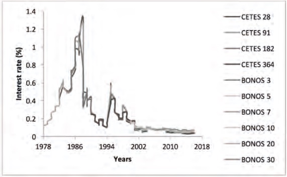
Table 1 shows the hypothesis tests to verify whether the series of time of the interest rates, in level and first difference, are stationary. The tests are also done for the GDP gap, the inflation rate, and the economic growth rate.
Table 1 Stationarity tests 1978-2017.
| Variable | Test statistics | |||||
|---|---|---|---|---|---|---|
| DFA | PP | KPSS | ||||
| Level | Difference | Level | Difference | Level | Difference | |
| CETES28 | -2.04 | -10.93*** | -1.97 | -13.08*** | 1.05*** | 0.06 |
| CETES91 | -1.59 | -10.76*** | -1.95 | -11.18*** | 1.04*** | 0.05 |
| CETES182 | -2.25 | -5.45*** | -1.78 | -7.93*** | 0.91*** | 0.04 |
| CETES364 | -1.74 | -9.40*** | -1.92 | -9.4*** | 0.89*** | 0.04 |
| BONOS3 | -2.71* | -8.18*** | -3.01** | -8.19*** | 0.88*** | 0.29 |
| BONOS5 | -3.52** | -6.84*** | -3.89*** | -6.83*** | 0.88*** | 0.48 |
| BONOS7 | -2.34 | -8.06*** | -2.30 | -9.20*** | 0.89*** | 0.21 |
| BONOS10 | -1.84 | -9.23*** | -1.73 | -9.75*** | 0.88*** | 0.12 |
| BONOS20 | -2.06 | -8.42*** | -1.96 | -9.99*** | 0.75*** | 0.11 |
| BONOS30 | -1.88 | -7.03*** | -1.92 | -7.03*** | 0.58*** | 0.06 |
| Level | Rate of change | Level | Rate of chance | Level | Rate of chance | |
| GDP | -3.63 | -16.95*** | -3.92 | -16.52*** | 1.06*** | 0.22 |
| INFLATION | -3.84 | -3.07*** | -3.69 | -2.94*** | 0.94*** | 0.15 |
| GAP | -4.18 | -3.311* | -3.88 | -3.24** | 0.88*** | 0.12 |
Source: Own elaboration with data from Banxico.
***: level of significance at 10%
***: level of significance at 5%
***: level of significance at 1%
It can be observed that under the Kwiatkowski-Phillips-Schmidt-Shin (KPSS) tests, the stationary hypothesis is not rejected, and that under the Augmented Dickey-Fuller (ADF) and Phillips-Perron (PP) tests, non-stationarity in levels is confirmed.
The results of Table 1 follow the observations presented by Lardic, Priaulet and Priaulet (2003), who argue in favor of the use of the first difference of the interest rates to do a multivariate analysis of the factor or principal components type. In this sense, the estimations of principal components are done using the correlation matrix of interest rate changes for the three subperiods: 1978-1988, 1989-2008 and 2009-2016. The correlation matrix is used as it allows reducing the bias of estimation attributable to the heterogeneous differences that exist in the interest rates observed according to their terms, Lardic, Priaulet and Priaulet (2003), Martínez and Núñez (2012).
To evaluate the relevance of the estimation by principal components, the Kaiser-Meyer-Ollin (KMO) criterion and Bartlett’s sphericity test (BS) are used. In this case, a regular sample adequacy level is shown for the first difference of the time series, as the KMO is slightly above 0.70. Furthermore, the null BS hypothesis is rejected, and it can be asserted that the variables are highly correlated (see Table 2).
Table 2 Sample adequacy for the application of PCA.
| 1978-1988 | 1989-2008 | 2009-2017 | |
|---|---|---|---|
| KMO | 0.7103 | 0.7120 | 0.7302 |
| EB | 57.032*** | 2238.513*** | 630.891*** |
| Normal multivariate | 56.616*** | 611.881*** | 22.388 |
Source: Own elaboration with data from Banxico.
*: level of significance at 10%
**: level of significance at 5%
***: level of significance at 1%.
Similarly, the Doornik-Hansen test is carried out to verify whether the variables behave like a multivariant normal (Mardia, Kent y Bibby, 1979) and it is found that only for the period of 2009-2016 the null hypothesis is not rejected. In this situation, calculations and inferences are done under the asymptotic approach indicated by Cuadras (2014) for the entire period of 1978-2017.
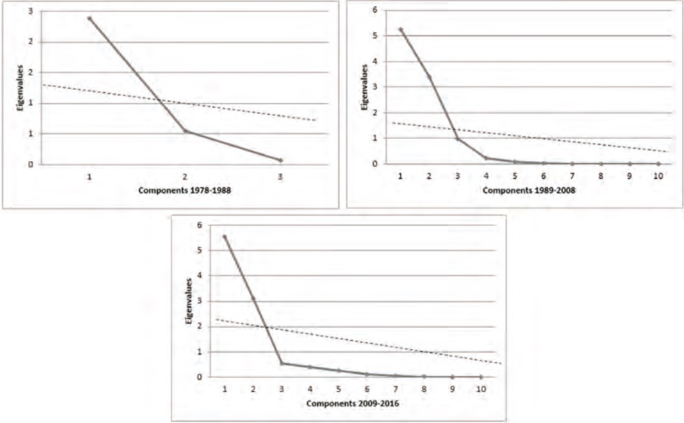
Table 3 shows the values of the two principal components that have been retained, according to the parallel simulation (PS) criterion (Dinno, 2009), see annexes. It could be indicated that the components chosen coincide with the values superior to the unit, as suggested by (Johnson and Wichern, 2000). The accumulated variation under the components is superior to 80% in each of the subperiods considered. In the first term, 1978-1988, only the first component is significant, according to PS, and only the first component has a value superior to the unit.
Table 3 Eigenvalues under PCA.
| 1978-1988 | 1989-2008 | 2009-2017 | ||||
|---|---|---|---|---|---|---|
| Accumulated variation | Eigen valores | Accumulated variation | Eigen valores | Accumulated variation | Eigen valores | Accumulated variation |
| Component 1 | 2.3561 | 78.540% | 5.2713 | 52.710% | 5.5416 | 55.429% |
| (1.90,3.49) | (5.60,6.36) | (4.50,7.96) | ||||
| Component 2 | 0.5943 | 98.350% | 3.3919 | 86.630% | 3.0930 | 86.365% |
| (0.48,0.88) | (2.96,4.09) | (2.51,4.44) | ||||
| Component 3 | 0.0496 | 100.000% | 0.9828 | 96.460% | 0.5418 | 91.785% |
| (0.04,0.08) | (0.86,1.19) | (0.44,0.78) | ||||
| Component 4 | 0.2282 | 98.740% | 0.3882 | 95.668% | ||
| (0.20,0.28) | (0.32,0.56) | |||||
| Component 5 | 0.0951 | 99.690% | 0.2394 | 98.062% | ||
| (0.08,0.11) | (0.19,0.34) | |||||
| Component 6 | 0.0182 | 99.870% | 0.1217 | 99.280% | ||
| (0.01,0.02) | (0.09,0.17) | |||||
| Component 7 | 0.0083 | 99.960% | 0.0587 | 99.866% | ||
| (0.007,0.010) | (0.05,0.08) | |||||
| Component 8 | 0.0026 | 99.980% | 0.0103 | 99.969% | ||
| (0.002,0.003) | (0.008,0.015) | |||||
| Component 9 | 0.0013 | 99.990% | 0.0029 | 99.999% | ||
| (0.001,0.002) | (0.0024,0.0042) | |||||
| Component 10 | 0.0004 | 100.000% | 0.0001 | 100.000% | ||
| (0.00008,0.00014) | ||||||
Source: Own elaboration with data from Banxico.
Table 4 shows the principal components retained for each of the subperiods, along with their confidence intervals at 95%. In the 1978-1988 term, only the first principal component is relevant, which suggests that in this period the significant part of the yield curve was only its level.
Table. 4 Granger causality
| Causation of Granger | ||||||||||||
|---|---|---|---|---|---|---|---|---|---|---|---|---|
| 1978-1988 | 1989-2008 | 2009-2017 | ||||||||||
| Null | 1 | 2 | 3 | 4 | 1 | 2 | 3 | 4 | 1 | 2 | 3 | 4 |
| hypotesis | Lag | Lag | Lag | Lag | Lag | Lag | Lag | Lag | Lag | Lag | Lag | Lag |
| GAP-C1 | × | × | × | × | × | × | × | × | ✓ | × | × | × |
| C1-GAP | ✓ | × | ✓ | ✓ | ✓ | ✓ | ✓ | ✓ | × | ✓ | ✓ | ✓ |
| GAP-C2 | × | × | × | ✓ | × | × | × | × | × | × | × | × |
| C2-GAP | × | × | × | × | ✓ | ✓ | ✓ | ✓ | × | × | × | × |
| INFLATION-C1 | × | × | × | × | × | × | × | × | × | × | × | × |
| C1-INFLATION | × | √ | × | × | ✓ | ✓ | × | ✓ | × | ✓ | ✓ | ✓ |
| INFLATION-C2 | × | × | ✓ | ✓ | × | × | × | ✓ | × | × | × | × |
| C2-INFLATION | ✓ | ✓ | ✓ | ✓ | × | × | × | × | × | × | × | × |
| GDP-C1 | × | × | × | × | × | × | × | × | ✓ | × | × | × |
| C1-GDP | × | × | × | × | × | ✓ | ✓ | ✓ | × | × | ✓ | ✓ |
| GDP-C2 | × | × | × | ✓ | × | × | × | × | ✓ | × | × | × |
| C2-GDP | × | × | × | × | ✓ | ✓ | ✓ | ✓ | × | × | × | × |
Source: Own elaboration with data from Banxico.
In turn, for the two subsequent subperiods, both the level and the slope of the curve are relevant, as their values are superior to the unit and they have statistical significance under PS.
The first principal component presents positive coefficients for the three terms of the 1978-2017 period, suggesting the interpretation of the first principal component as the “level” of the yield curve, since it can be seen as a “weighted average”, while for 1978-1988 the most relevant rate is CETES at 91 days. Meanwhile, for 1989-2017 the most important rates are CETES at 364 days and Bonds at 3, 5 and 7 years.
The second principal component has positive and negative coefficients, which indicates that the interest rates have a differentiated influence on the yield curve. During the 1989-2008 term the CETES interest rates at 28, 91, 182 and 364 days have a positive influence, while the bond rates at 3, 5, 7, 10, 20 and 30 years contribute negatively. In contrast, in recent years, 2009-2016, the behavior is different, as the it is the bond rates at 3, 5, 7, 10 20 and 30 years that positively contribute to the slope of the yield curve.
Using the estimated variables, the Granger causality test is done between the economic growth rate, the inflation rate, the GDP gap, and the principal components of each subperiod. Table 4 indicates with a checkmark the case where the null hypothesis was rejected, and which provides evidence of causality between the variables. The set of all of the test statistics and p values are presented in the annexes.
Based on Table 4, there is evidence to assert that the first (C1) and second (C2) components cause a product gap, inflation rate and economic growth rates, although to a lesser extent, as only the results for 1989 and thereafter are observable. This last finding is similar to the estimations by Cerecero, Salazar and Salgado (2008), Castellanos and Camero (2003), who carried out similar exercises with the differentials of the interest rates.
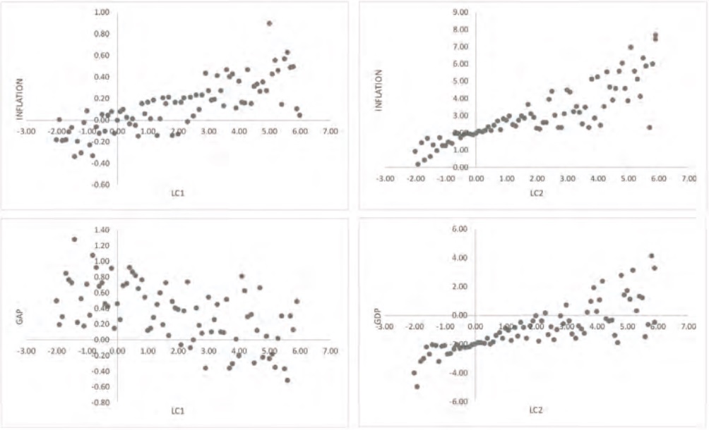
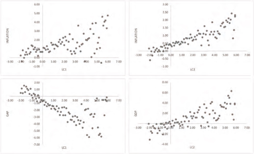
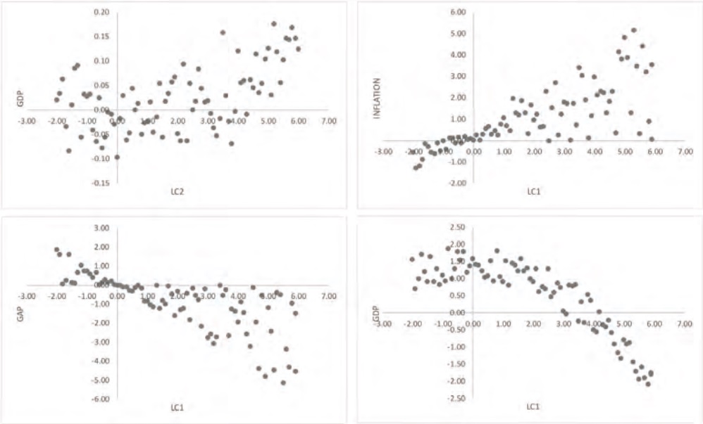
Figure 4 (see annexes) shows the dispersion diagrams between the variables GAP, INFLATION and GDP against components C1 and C2 for each subperiod, according to the evidence found for Granger causality.
The graphs from Figure 4 attempt to show those patterns that are visually direct, as a solid argument can be found through Granger causality tests and vector autoregression, where the endogeneity and temporality of the involved variables are considered.
Figure 4a (period 1978-1988) shows that when C1 is negative, the GAP increases and when C1 is positive, the GAP decreases. Higher levels of the C1 variable tend to close the GDP gap. In turn, when C1 increases, INFLATION tends to rise. The GDP tends to decrease when C2 increases. Given the usual interpretation of C1 (Martínez and Núñez, 2012), the graphs suggest that the level of the yield curve positively affects the inflation rate. While component C2, associated to the slope of the yield curve, negatively affects the GDP variable.
Figure 4b (period 1989-2008) the GAP variable inversely relates to C1, while C1 directly and positively affects INFLATION. The C2 component also positively affects the inflation rate and the economic growth rate.
It can be observed in Figure 4 of the annex that the second component has a positive relation to the economic growth rate. This indicates that with a greater expiration rate in the long-term there is a positive effect when compared to the short-term rates.
Table 5 shows the estimated coefficients of the principal components within a VAR model which endogenously relates the macroeconomic variables with C1 and C2 (see annex). The optimal number of lag, according to the information criteria by Akaike and Schwarz, are reported in the annexes and are equal to four quarters.
Table 5 Coefficients of the VAR model in 1978-2017.
| GDP | INFLATION | GAP | C1 | C2 | |
|---|---|---|---|---|---|
| C1(-1) | -0.0107 | 0.0194 | -0.0118 | 1.2224 | -0.0226 |
| (0.0049) | (0.007) | (0.0049) | (0.041) | (0.0489) | |
| [-2.1944] | [2.7871] | [-2.4218] | [11.7417] | [-0.4624] | |
| C1(-2) | 0.0118 | -0.0180 | 0.0141 | -0.6999 | 0.1269 |
| (0.0069) | (0.0099) | (0.0069) | (0.1481) | (0.0695) | |
| [1.708] | [-1.8204] | [2.0339] | [-4.7272] | [1.8252] | |
| C1(-3) | -0.0093 | 0.0255 | -0.0101 | 0.6083 | 0.0148 |
| (0.007) | (0.01) | (0.007) | (0.1491) | (0.07) | |
| [-1.3399] | [2.5639] | [-1.4536] | [4.0805] | [0.212] | |
| C1(-4) | 0.0033 | -0.0147 | 0.0038 | -0.2090 | -0.0624 |
| (0.0048) | (0.0068) | (0.0048) | (0.1019) | (0.0478) | |
| [0.6996] | [-2.155] | [0.7994] | [-2.0517] | [-1.305] | |
| C2(-1) | 0.0015 | 0.0908 | 0.0006 | 1.8711 | 0.2372 |
| (0.0086) | (0.0123) | (0.0086) | (0.1832) | (0.0861) | |
| [0.1739] | [7.4146] | [0.0749] | [10.2073] | [2.7556] | |
| C2(-2) | 0.0269 | -0.0230 | 0.0294 | -1.1463 | 0.1713 |
| (0.0115) | (0.0165) | (0.0115) | (0.2471) | (0.116) | |
| [2.3341] | [-1.3959] | [2.5513] | [-4.6384] | [1.4766] | |
| C2(-3) | -0.0022 | 0.0468 | -0.0034 | 0.6100 | -0.2102 |
| (0.0122) | (0.0175) | (0.0122) | (0.2613) | (0.1227) | |
| [-0.1823] | [2.6801] | [-0.2819] | [2.3347] | [-1.7136] | |
| C2(-4) | -0.0175 | -0.0367 | -0.0112 | -1.0496 | -0.3132 |
| (0.0117) | (0.0168) | (0.0117) | (0.2514) | (0.118) | |
| [-1.49] | [-2.185] | [-0.951] | [-4.1759] | [-2.6543] |
Source: Own elaboration with data from Banxico.
*: level of significance at 10%
**: level of significance at 5%
***: level of significance at 1%
The estimated coefficients (Table 5) represent, in each case, the impact that the variation of the principal component has on the economic growth rate, the GDP gap, and the inflation rate. It can be observed that the principal component associated to the level of the yield curve (C1) presents a significant negative impact on the GDP, which intuitively indicates that if the level of the interest rates rises, then there will be a reverse effect on the economic growth rate. Conversely, a change of one unit in the main component associated to the slope of the yield curve (C2) has a positive effect, indicating that with a higher differential between short and long-term interest there will be a positive effect on the economic growth rate. This last result is similar to what was indicated by Cerecero, Salazar and Salgado (2008) and Castellanos and Camero (2003).
Regarding the impact on the GAP variable, there is evidence of Granger causality in the three stationary growth subperiods, although the period from 1989-2008 stands out, where both components are relevant throughout four quarters of lag, see Table 4. If the VAR model coefficients are considered, then there will be positive and negative coefficients. Given that the GAP variable is defined as the percentage change between the potential GDP and the real GDP of the period, then components C1 and C2 close the gap of the product, see Table 5.
In the case of the INFLATION variable, positive and negative signs in the coefficients of components C1 and C2 are also observed, see Table 5. However, the biggest effect is positive, and so components C1 and C2 contribute in an upwards manner to the inflation rate. Similarly, Table 4 presents evidence of Granger causality, particularly in the subperiod of 1978-1988.
In general, there has been evidence of Granger causality for the three variables, GAP, INFLATION and GDP, and for the VAR model there is evidence of significant impacts of the principal components, which are associated with the level and slope of the yield curve.
That said, Table 6 shows the variance decomposition of the VAR model where it can be appreciated that components C1 and C2 contribute to the variation of the GDP, GAP and INFLATION in at least 2% of quarters 1, 4, 8 and 12 of the estimation. The total set of estimations cab be seen in the annexes, observing the same behavior for the remaining quarters of the 1978-2017 period.
Table 6 Variance decomposition.
| Decomposition of variancde: GDP | ||||||
|---|---|---|---|---|---|---|
| Period | Standard error | GDP | INFLATION | GAP | C1 | C2 |
| 1 | 0.0154 | 100 | 0.0000 | 0.0000 | 0.0000 | 0.0000 |
| 4 | 0.0171 | 89.9307 | 4.2836 | 2.7928 | 2.9155 | 0.0774 |
| 8 | 0.0203 | 85.9748 | 4.3048 | 2.8316 | 3.5114 | 3.3773 |
| 12 | 0.0219 | 85.5181 | 4.3998 | 2.7579 | 3.4910 | 3.8332 |
| Decomposition of variance: INFLATION | ||||||
| Period | Standard error | GDP | INFLATION | GAP | C1 | C2 |
| 1 | 0.0154 | 100 | 0.0000 | 0.0000 | 0.0000 | 0.0000 |
| 4 | 0.0171 | 89.9307 | 4.2836 | 2.7928 | 2.9155 | 0.0774 |
| 8 | 0.0203 | 85.9748 | 4.3048 | 2.8316 | 3.5114 | 3.3773 |
| 12 | 0.0219 | 85.5181 | 4.3998 | 2.7579 | 3.4910 | 3.8332 |
| Descomposition of variance GAP | ||||||
| Period | Standard error | GDP | INFLATION | GAP | C1 | C2 |
| 1 | 0.0154 | 100 | 0.0000 | 0.0000 | 0.0000 | 0.0000 |
| 4 | 0.0171 | 89.9307 | 4.2836 | 2.7928 | 2.9155 | 0.0774 |
| 8 | 0.0203 | 85.9748 | 4.3048 | 2.8316 | 3.5114 | 3.3773 |
| 12 | 0.0219 | 85.5181 | 4.3998 | 2.7579 | 3.4910 | 3.8332 |
In graphical terms, Figure 2 shows the functions of impulse and response for the macroeconomic variables and components C1 and C2. It can be appreciated that for the case of the GAP variable, the response is lower than zero and the components contribute to the closing of the product gap.
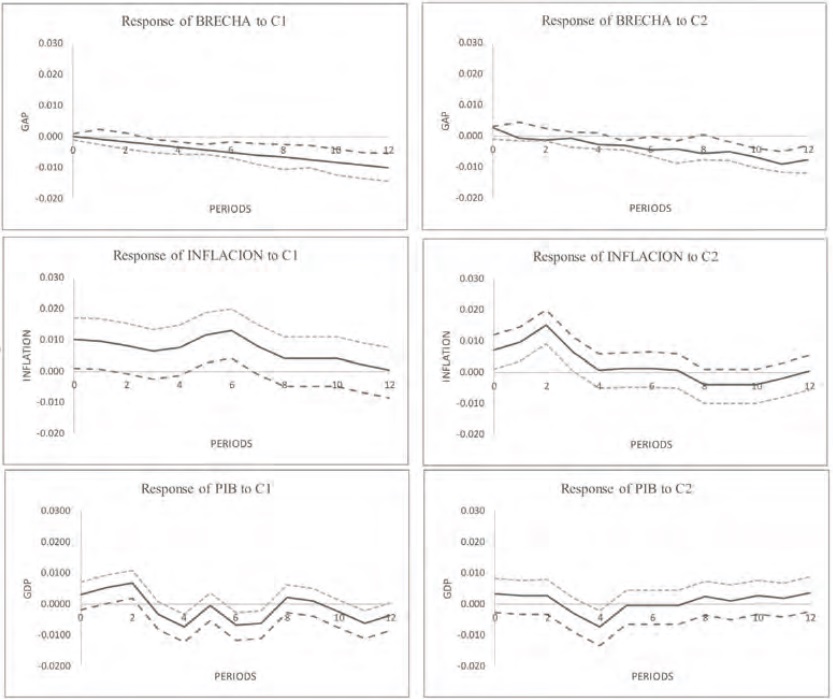
When the graphs for the INFLATION variable are observed, it can be observed that C1 has a positive effect, which contributes to the rising of the inflation rate throughout the 12 indicated quarters. While C2 increases the inflation rate in the short-term, it has a negative influence in the long-term. That is, component C1, associated to the slope of the yield curve, contributes to the increase of the inflation rate in the short-term and its decrease in the long-term.
Finally, the effect of component C1 on the economic growth rate is oscillatory, as the answer of the GDP to increase and decrease around the initial point, although it is biased in a downward manner, that is, an increase in C1 tends to decrease the GDP variable. While the C2 component slightly increases the GDP variable, a fall can be seen afterwards, and in the long-term there is a positive effect.
Conclusions
This work finds evidence to assert that the dynamic of the yield curve can be studied through two variables (principal components) for each of the three subperiods: 1978-1988, 1989-2008 and 2009-2017. The factors found are consistent with those cited in the literature and which are usually associated with the level and the slope of the yield curve, as stated in Martínez and Núñez (2012), Cortés, Ramos and Torres (2009) and Jiménez (2002). In the subperiod of 1978-1988, only the first principal component is relevant and explains 78.54% of the variation of the interest rates-all the coefficients are superior to zero. In this case, the PCA only finds the level of the yield curve relevant, according to the parallel simulation criterion, see Figure 3 in the annex.
In the years of 1989-2008 and 2009-2016 the first two principal components are significant; they gather 86.63% and 86.37% of the variation of the interest rates, respectively. In these periods, both the level and the slope of the yield curve are relevant, with the bond rates at 3, 5, 7, 10, 20, and 30 years positively contributing to the slope of the curve in 2009-2017, in contrast to subperiod 1989-2008.
There was evidence of Granger causality in each subperiod of components C1 and C2 on the economic growth rates, inflation rate, and product gap variables. These results are ratified in the estimated VAR model, where differentiated effects of components C1 and C2 can be observed. Through the impulse and response functions it is found that components C1 and C2 contribute to the closing of the product gap. While for the case of the INFLATION variable, the C1 variable has a positive contribution, whereas C2 increases the inflation rate in the short-term but has a negative influence in the long-term. Now, when observing the economic growth rate, the effect of component C1 is oscillatory, although with a downwards bias; that is, an increase in C1 tends to decrease the GDP variable, but at the same time, the C2 component increases the GDP variable in a long-term horizon.
This last result is consistent with the positive effect that a change in the slope of the yield curve has on the economic activity, as indicated in Cerecero, Salazar and Salgado (2008) y Castellanos and Camero (2003).
Finally, it can be pointed out that the effects of C1 and C2 reflect a set of latent factors, the movement of which is predictive of the economic activity. In this sense, the exercise presented in this document attempts to build a bridge between the real sector of the economy and the movements of the financial variables.
REFERENCES
Ang, A. y Piazzesi, M. (2003). A No-Arbitrage Vector Autoregression of Term Structure Dynamics with macroeconomics and Latent variables. Journal of Monetary Economics, 50, 745-787. https://doi.org/10.1016/s0304-3932(03)00032-1 [ Links ]
Barber, J. y Cooper, M. (1996). Immunization Using Principal Component Analysis. Journal of Portfolio Management, 23 (1), 99-105. https://doi.org/10.3905/jpm.1996.409574 [ Links ]
Bühler, A. y Zimmermann (1996). A statistical analysis of the term structure of interest rates in Switzerland and Germany, Journal of Fixed Income, 6(3), 55-67. https://doi.org/10.3905/jfi.1996.408182 [ Links ]
Castellanos, S.G. y Camero, E. (2003). La estructura temporal de las tasas de interés en México: ¿puede ésta predecir la actividad económica futura? Revista de Análisis Económico, 18 (2), 37-52. Disponible en: http://repositorio.uahurtado.cl/handle/11242/1790 Consultado: 13/05/2016 [ Links ]
Cerecero, M., Salazar, C. D. y Salgado, B. H. (2008). La curva de rendimiento y su relación con la actividad económica: una aplicación para México. Working paper, Banco de México. Disponible en: https://www.econstor.eu/handle/10419/83775 Consultado: 15/04/2016 [ Links ]
Cortés, J., Ramos M. y Torres A. (2009). An Empirical Analysis of the Mexican Term Structure of Interest Rate. Economics Bulletin, 29 (3), 2310-2323. Disponible en: https://core.ac.uk/download/pdf/6442917.pdf Consultado: 27/03/2016 [ Links ]
Cuadras, C. (2014). Nuevos métodos de análisis multivariante, Manacor, Barcelona, España. Disponible en: http://www.ub.edu/stat/personal/cuadras/metodos.pdf Consultado: 12/05/2016 [ Links ]
D’Ecclesia, R.L. and Zenios, S. A. (1994). Risk Factor Analysis and Portfolio Immunization in the Italian Bond Market. Journal of Fixed Income 4(29), 51-58. https://doi.org/10.3905/jfi.1994.408113 [ Links ]
Dinno, A. (2009). Implementing Horn’s parallel analysis for principal component analysis and factor analysis. Stata Journal, 9 (2), 291-302. Disponible en: https://www.stata-journal.com/article.html?article=st0166 Consultado: 11/06/2016 [ Links ]
Enders, W. (2004). Applied Econometric Time Series, 2a. ed., John Wiley & Sons, Inc. [ Links ]
García, V. S. (2011). Algunas consideraciones sobre la estructura temporal de tasas de interés del gobierno en México (No. 2011-18). Working Papers, Banco de México. Disponible en: https://www.econstor.eu/handle/10419/83698 Consultado: 10/03/2016 [ Links ]
Greene, W.H. (2010). Econometric Analysis, 5a. ed., Prentice Hall, New Jersey. [ Links ]
Jiménez, V. (2002) Testing the stability of the Components Explaining Changes of the Yield Curve in Mexico. A principal Component Analysis Approach. Trans 27th ICA. Disponible en: https://pdfs.semanticscholar.org/7760/5bb62c251124c19968e2f883d12d5816c850.pdf Consultado: 17/02/2016 [ Links ]
Johnson, R. y Wichern, D. (2000). Applied multivariate statistical analysis. Vol. 5. Englewood Cliffs, NJ: Prentice Hall. [ Links ]
Knez, J., Litterman R. y Scheinkman, J. (1996). Exploration into Factors Explaining Money Market Returns. Journal of Finance, 49(5), 1861-1881. https://doi.org/10.2307/2329274 [ Links ]
Lardic, S., Priaulet, P. y Priaulet, S. (2003). PCA of the Yield Curve Dynamics: Questions of Methodologies, Journal of Bond Trading and Management, 1(4), 327-349. [ Links ]
Litterman, R. y Scheinkman, J. (1991). Common Factors Affecting Bond Returns. Journal of Fixed Income, 1, 54-61. https://doi.org/10.3905/jfi.1991.692347 [ Links ]
Martínez, C. y Núñez, J.A. (2012). Análisis de componentes principales de la estructura a plazos de las tasas de interés en México. eseconomia, VII (33), 3-23. Disponible en: http://yuss.me/revistas/ese/ese2012v07n33a01p003_023.pdf . Consultado: 14/04/2016 [ Links ]
Mardia, K. V., Kent, J. T. y Bibby, J. M. (1979). Multivariate analysis. 1a. ed., New York, Academy Press. [ Links ]
Noriega, A. y Rodríguez-Peréz, C.A. (2011). Estacionariedad, Cambios Estructurales y Crecimiento Económico en México: 1895-2008. Documento de Trabajo, Banco de México. [ Links ]
Redington, F.M. (1952). Review of the Principle of Life Office Valuations. Journal of the Institute of Actuaries, 78 (1), 286-340. [ Links ]
Annexes
A. Principal components and parallel simulation, 1978-2017
| 1978-1988 | 1989-2008 | 2009-2012 | ||||
|---|---|---|---|---|---|---|
| Component 1 | Component 2 | Component 1 | Component 2 | Component 1 | Component 2 | |
| DCETES28 | 0.596 | -0.559 | 0.134 | 0.502 | 0.282 | -0.386 |
| (0.573,0.619) | (-0.629,-0.587) | (0.132,0.135) | (0.485,0.518) | (0.277,0.288) | (-0.396,-0.377) | |
| DCETES91 | 0.626 | -0.233 | 0.171 | 0.485 | 0.306 | -0.380 |
| (0.601,0.651) | (-0.301,0.217) | (0.169,0.173) | (0.470,0.501) | (0.301,0.313) | (-0.388,-0.370) | |
| DCETES182 | 0.504 | 0.796 | 0.268 | 0.419 | 0.334 | -0.345 |
| (0.487,0.52) | (0.564,0.897) | (0.264,0.173) | (0.408,0.431) | (0.327,0.341) | (-0.353,-0.338) | |
| DCETES364 | 0.334 | 0.322 | 0.353 | -0.295 | ||
| (0.327,0.341) | (0.315,0.329) | (0.346,0.362) | (-0.298,-0.287) | |||
| DBONOS3 | 0.381 | -0.098 | 0.365 | 0.049 | ||
| (0.371,0.390) | (-0.099,-0.097) | (0.356,0.373) | (0.049,0.049) | |||
| DBONOS5 | 0.393 | -0.137 | 0.349 | 0.150 | ||
| (0.383,0.403) | (-0.139,-0.136) | (0.342,0.358) | (0.148,0.151) | |||
| DBONOS7 | 0.401 | -0.144 | 0.361 | 0.274 | ||
| (0.391,0.412) | (-0.146,-0.143) | (0.352,0.369) | (0.270,0.279) | |||
| DBONOS10 | 0.393 | -0.166 | 0.276 | 0.323 | ||
| (0.383,0.403) | (-0.168,-0.165) | (0.269,0.279) | (0.317,0.330) | |||
| DBONOS20 | 0.283 | -0.274 | 0.300 | 0.342 | ||
| (0.277,0.288) | (-0.279,-0.269) | (0.294,0.305) | (0.336,0.351) | |||
| DBONOS30 | 0.273 | -0.285 | 0.198 | 0.423 | ||
| (0.268,0.278) | (-0.29,-0.279) | (0.195,0.200) | (0.412,0.435) | |||
Source: Own elaboration with data from Banxico.
B. Granger causality tests.
| Granger’s causality: 1 lag | ||||||||
|---|---|---|---|---|---|---|---|---|
| 1978-1988 | 198-2008 | 2009-2017 | ||||||
| Null hypothesis | Statistic F | p value | Null hypothesis | Statistic F | p value | Null hypothesis | Statistic F | p value |
| GAP-C1 | 0.9722 | 0.3301 | GAP-C1 | 0.0622 | 0.8037 | GAP-C1 | 15.3815 | 0.0005 |
| C1-GAP | 35.9317 | 0.0000 | C1-GAP | 8.8610 | 0.0039 | C1-GAP | 2.5148 | 0.1229 |
| GAP-C2 | 0.7895 | 0.3796 | GAP-C2 | 2.1099 | 0.1504 | GAP-C2 | 0.8677 | 0.3588 |
| C2-GAP | 0.0658 | 0.7988 | C2-GAP | 8.2687 | 0.0052 | C2-GAP | 0.1059 | 0.7471 |
| INFLATION-C1 | 0.4740 | 0.4951 | INFLATION-C1 | 1.1895 | 0.2788 | INFLATION-C1 | 0.9919 | 0.3270 |
| C1-INFLATION | 2.5267 | 0.2298 | C1-INFLATION | 6.1084 | 0.0157 | C1-INFLATION | 0.0002 | 0.9877 |
| INFLATION-C2 | 1.1669 | 0.2865 | INFLATION-C2 | 0.3733 | 0.5430 | INFLATION-C2 | 0.0130 | 0.9099 |
| C2-INFLATION | 55.5878 | 0.0000 | C2-INFLATION | 0.1106 | 0.7403 | C2-INFLATION | 0.0182 | 0.8937 |
| GDP-C1 | 2.6708 | 0.1101 | GDP-C1 | 0.4088 | 0.5245 | GDP-C1 | 3.0280 | 0.0918 |
| C1-GDP | 0.3328 | 0.5673 | C1-GDP | 0.0005 | 0.9433 | C1-GDP | 1.0125 | 0.3221 |
| GDP-C2 | 0.0592 | 0.8091 | GDP-C2 | 0.0576 | 0.8110 | GDP-C2 | 5.5648 | 0.0248 |
| C2-GDP | 0.0072 | 0.9330 | C2-GDP | 13.9274 | 0.0004 | C2-GDP | 0.2791 | 0.6011 |
Source: Own elaboration with data from Banxico.
| Granger’s causality: 2 lags | ||||||||
|---|---|---|---|---|---|---|---|---|
| 1978-1988 | 198-2008 | 2009-2017 | ||||||
| Null hypothesis | Statistic F | p value | Null hypothesis | Statistic F | p value | Null hypothesis | Statistic F | p value |
| GAP-C1 | 0.8693 | 0.4276 | GAP-C1 | 0.2228 | 0.8008 | GAP-C1 | 2.2590 | 0.1225 |
| C1-GAP | 0.0276 | 0.1460 | C1-GAP | 9.9806 | 0.0001 | C1-GAP | 3.1383 | 0.0584 |
| GAP-C2 | 0.6781 | 0.5138 | GAP-C2 | 0.8879 | 0.4158 | GAP-C2 | 1.8234 | 0.1795 |
| C2-GAP | 0.1816 | 0.8347 | C2-GAP | 9.3441 | 0.0002 | C2-GAP | 1.6720 | 0.2055 |
| INFLATION-C1 | 1.1194 | 0.3373 | INFLATION-C1 | 0.9318 | 0.3984 | INFLATION-C1 | 0.7465 | 0.4829 |
| C1-INFLATION | 2.6453 | 0.0844 | C1-INFLATION | 4.4844 | 0.0145 | C1-INFLATION | 2.9405 | 0.0687 |
| INFLATION-C2 | 1.0900 | 0.3468 | INFLATION-C2 | 2.0422 | 0.1369 | INFLATION-C2 | 1.5773 | 0.2237 |
| C2-INFLATION | 23.7165 | 0.0000 | C2-INFLATION | 0.3045 | 0.7384 | C2-INFLATION | 0.4619 | 0.6347 |
| GDP-C1 | 1.4995 | 0.2365 | GDP-C1 | 0.3637 | 0.6963 | GDP-C1 | 2.2338 | 0.1252 |
| C1-GDP | 0.2953 | 0.7461 | C1-GDP | 9.7559 | 0.0002 | C1-GDP | 0.8714 | 0.4290 |
| GDP-C2 | 0.0860 | 0.9178 | GDP-C2 | 0.0934 | 0.9109 | GDP-C2 | 2.2972 | 0.1185 |
| C2-GDP | 0.0519 | 0.9495 | C2-GDP | 7.1049 | 0.0015 | C2-GDP | 2.3835 | 0.1101 |
Source: Own elaboration with data from Banxico.
| Granger's causality: 3 lags | ||||||||
|---|---|---|---|---|---|---|---|---|
| 1978-1988 | 198-2008 | 2009-2017 | ||||||
| Null hypotesis | Statistic F | p Value | Null hypotesis | Statistic F | p Value | Null hypotesis | Statistic F | p Value |
| GAP-C1 | 0.6506 | 0.5881 | GAP-C1 | 0.1513 | 0.9286 | GAP-C1 | 1.4325 | 0.2551 |
| C1-GAP | 2.3785 | 0.0869 | C1-GAP | 6.9721 | 0.0003 | C1-GAP | 2.6485 | 0.0691 |
| GAP-C2 | 0.6560 | 0.5848 | GAP-C2 | 0.4032 | 0.7511 | GAP-C2 | 1.5012 | 0.2367 |
| C2-GAP | 0.1329 | 0.9398 | C2-GAP | 5.9197 | 0.0011 | C2-GAP | 1.6723 | 0.1964 |
| INFLATION-C1 | 0.6101 | 0.6131 | INFLATION-C1 | 0.3570 | 0.7842 | INFLATIO-C1 | 1.1759 | 0.3373 |
| C1-INFLATION | 1.4871 | 0.2355 | C1-INFLATION | 1.0179 | 0.3898 | C1-INFLATION | 6.2737 | 0.0023 |
| INFLATION-C2 | 3.4626 | 0.0268 | INFLATIO-C2 | 1.1257 | 0.3444 | INFLATION-C2 | 0.9877 | 0.4133 |
| C2-INFLATION | 14.3284 | 0.0000 | C2-INFLATION | 0.2710 | 0.8461 | C2-INFLATION | 0.5136 | 0.6763 |
| GDP-C1 | 0.8236 | 0.4900 | GDP-C1 | 0.4867 | 0.6926 | GDP-C1 | 1.7420 | 0.1821 |
| C1-GDP | 0.2859 | 0.8352 | C1-GDP | 7.5425 | 0.0002 | C1-GDP | 2.3443 | 0.0953 |
| GDP-C2 | 0.0986 | 0.9602 | GDP-C2 | 0.3753 | 0.7711 | GDP-C2 | 1.5029 | 0.2362 |
| C2-GDP | 0.0464 | 0.9865 | C2-GDP | 5.6100 | 0.0016 | C2-GDP | 0.6663 | 0.5801 |
Source: Own elaboration with data from Banxico.
| Granger’s causality: 4 lags | ||||||||
|---|---|---|---|---|---|---|---|---|
| 1978-1988 | 198-2008 | 2009-2017 | ||||||
| Null hypotesis | Statistic F | p value | Null hypotesis | Statistic F | p value | Null hypotesis | Statistic F | p value |
| GAP-C1 | 0.9894 | 0.4279 | GAP-C1 | 0.3322 | 0.8554 | GAP-C1 | 1.2188 | 0.3279 |
| C1-GAP | 2.3707 | 0.0740 | C1-GAP | 4.9802 | 0.0014 | C1-GAP | 17.6800 | 0.0000 |
| GAP-C2 | 3.9589 | 0.0104 | GAP-C2 | 0.3935 | 0.8127 | GAP-C2 | 0.8131 | 0.5288 |
| C2-GAP | 0.6610 | 0.6237 | C2-GAP | 5.0741 | 0.0012 | C2-GAP | 1.5719 | 0.2126 |
| INFLATION-C1 | 0.7420 | 0.5706 | INFLATION-C1 | 0.5815 | 0.6770 | INFLATION-C1 | 0.8804 | 0.4897 |
| C1-INFLATION | 1.3193 | 0.2847 | C1-INFLATION | 2.1854 | 0.0793 | C1-INFLATION | 3.6389 | 0.0181 |
| INFLATION-C2 | 4.2355 | 0.0075 | INFLATION-C2 | 2.3770 | 0.0600 | INFLATION-C2 | 0.7815 | 0.5479 |
| C2-INFLATION | 10.8255 | 0.0000 | C2-INFLATION | 0.3285 | 0.8580 | C2-INFLATION | 1.1734 | 0.3464 |
| GDP-C1 | 1.1262 | 0.3622 | GDP-C1 | 0.7552 | 0.5579 | GDP-C1 | 1.3369 | 0.2839 |
| C1-GDP | 0.2548 | 0.9045 | C1-GDP | 5.2230 | 0.0010 | C1-GDP | 5.8163 | 0.0019 |
| GDP-C2 | 2.4459 | 0.0672 | GDP-C2 | 0.9090 | 0.4635 | GDP-C2 | 0.8601 | 0.5013 |
| C2-GDP | 0.0582 | 0.9934 | C2-GDP | 5.4923 | 0.0007 | C2-GDP | 1.9135 | 0.1395 |
Source: Own elaboration with data from Banxico.
C. VAR Optimal lags, 1978-2017.
| Lags | LL | LR | FPE | AIC | HQIC | SBIC |
|---|---|---|---|---|---|---|
| 0 | 262.85 | 7.10E-11 | -14.8484 | -14.8024 | -14.7151 | |
| 1 | 412.09 | 298.480 | 2.40E-14 | -22.8622 | -22.6781 | -22.3290 |
| 2 | 438.70 | 53.223 | 8.80E-15 | -23.8686 | -23.5464 | -22.9354* |
| 3 | 451.74 | 26.070 | 7.20E-15 | -24.0992 | -23.6389 | -22.7660 |
| 4 | 466.45 | 29.432* | 5.5E-15* | -24.4258* | -23.8275* | -22.6927 |
Source: Own elaboration with data from Banxico.
LL: Log-likelihood
LR: Likelihood ratio
FPE: Final Prediction Error.
AIC: Akaike information criterion.
HQIC: Hanna-Quinn information criterion.
SBIC: Schwarz information criterion.
*: level of significance at 10%
**: level of significance at 5%
***: level of significance at 1%.
D. Variance decomposition.
| Decomposition of variance: GDP | ||||||
|---|---|---|---|---|---|---|
| Period | Standard error | GDP | INFLATION | GAP | C1 | C2 |
| 1 | 0.0154 | 100 | 0.0000 | 0.0000 | 0.0000 | 0.0000 |
| (0.0000) | (0.0000) | (0.0000) | (0.0000) | (0.0000) | ||
| 2 | 0.0160 | 92.81721 | 3.213212 | 1.007402 | 2.942869 | 0.019305 |
| (4.0493) | (2.72) | (1.9153) | (2.6465) | (0.9655) | ||
| 3 | 0.0161 | 91.93771 | 4.019095 | 1.05264 | 2.90392 | 0.086631 |
| (4.3687) | (3.0727) | (2.106) | (2.6313) | (1.3073) | ||
| 4 | 0.0171 | 89.93068 | 4.283624 | 2.792818 | 2.915526 | 0.077354 |
| (4.5848) | (2.9392) | (2.7937) | (2.439) | (1.3382) | ||
| 5 | 0.0189 | 87.66972 | 3.761524 | 2.315443 | 2.444326 | 3.808984 |
| (4.931) | (2.7416) | (2.3949) | (2.1916) | (2.7319) | ||
| 6 | 0.0194 | 86.82715 | 3.774256 | 2.376519 | 3.378141 | 3.646968 |
| (5.1763) | (2.8579) | (2.4469) | (2.7309) | (2.6977) | ||
| 7 | 0.0195 | 86.22979 | 4.416794 | 2.355332 | 3.354963 | 3.64312 |
| (5.4556) | (3.1962) | (2.4734) | (2.7953) | (2.6862) | ||
| 8 | 0.203 | 85.97481 | 4.304811 | 2.831617 | 3.511419 | 3.37734 |
| (5.5854) | (3.1383) | (2.661) | (2.6759) | (2.5723) | ||
| 9 | 0.0208 | 86.01843 | 4.496545 | 2.701905 | 3.400706 | 3.382417 |
| (5.6212) | (3.2406) | (2.5821) | (2.6931) | (2.6042) | ||
| 10 | 0.0212 | 85.77206 | 4.35565 | 2.697794 | 3.610945 | 3.563553 |
| (5.7398) | (3.2073) | (2.5656) | (2.8302) | (2.6868) | ||
| 11 | 0.0213 | 85.32581 | 4.505913 | 2.74503 | 3.68886 | 3.734387 |
| (5.9517) | (3.3494) | (2.6746) | (2.9415) | (2.7754) | ||
| 12 | 0.0219 | 85.51805 | 4.399798 | 2.757884 | 3.491041 | 3.833227 |
| (5.9873) | (3.2936) | (2.6981) | (2.8382) | (2.8641) | ||
| Decomposition of variance: INFLATION | ||||||
|---|---|---|---|---|---|---|
| Period | Standard error | GDP | INFLATION | GAP | C1 | C2 |
| 1 | 0.0154 | 100 | 0.0000 | 0.0000 | 0.0000 | 0.0000 |
| (4.3934) | (4.3934) | (0.0000) | (0.0000) | (0.0000) | ||
| 2 | 0.0160 | 92.81721 | 3.213212 | 1.007402 | 2.942869 | 0.019305 |
| (3.4929) | (5.9987) | (0.8409) | (1.107) | (5.1254) | ||
| 3 | 0.0161 | 91.93771 | 4.019295 | 1.05264 | 2.90392 | 0.086631 |
| (3.4473) | (7.0795) | (2.8409) | (1.4357) | (6.8714) | ||
| 4 | 0.0171 | 89.93068 | 4.283624 | 2.792818 | 2.915526 | 0.077354 |
| (3.5707) | (7.0396) | (3.6621) | (2.6277) | (7.3256) | ||
| 5 | 0.0189 | 87.66972 | 3.761524 | 2.315443 | 2.444326 | 3.808984 |
| (3.6529) | (6.7277) | (3.6253) | (4.6978) | (7.4491) | ||
| 6 | 0.0194 | 86.82715 | 3.774256 | 2.376519 | 3.378141 | 3.643938 |
| (3.5967) | (6.7681) | (3.9767) | (5.6595) | (6.9861) | ||
| 7 | 0.0195 | 86.22979 | 4.416794 | 2.355332 | 3.359463 | 3.64312 |
| (3.9066) | (6.9987) | (4.4903) | (5.9587) | (6.6795) | ||
| 8 | 0.203 | 85.97481 | 4.304811 | 2.831617 | 2.831617 | 3.400706 |
| (4.0802) | (7.1023) | (4.7302) | (6.22) | (6.554) | ||
| 9 | 0.0208 | 86.01843 | 4.496545 | 2.701905 | 3.400706 | 3.382417 |
| (3.9943) | (7.1415) | (4.7599) | (6.2865) | (6.5909) | ||
| 10 | 0.0212 | 85.77206 | 4.35565 | 2.697794 | 3.610945 | 3.563553 |
| (4.0769) | (7.1614) | (4.771) | (6.4884) | (6.6665) | ||
| 11 | 0.0213 | 85.32581 | 4.505913 | 2.74503 | 3.68886 | 3.734387 |
| (4.2604) | (7.1597) | (4.772) | (6.1918) | (6.6688) | ||
| 12 | 0.0219 | 85.51805 | 4.399798 | 2.757884 | 3.491041 | 3.833227 |
| (4.4346) | (7.1364) | (4.7512) | (6.1368) | (6.6521) | ||
| Decomposition of variance: GAP | ||||||
|---|---|---|---|---|---|---|
| Period | Standard error | GDP | INFLATION | GAP | C1 | C2 |
| 1 | 0.0154 | 100 | 0.0000 | 0.0000 | 0.0000 | 0.0000 |
| (1.1953) | (0.1082) | (0.1828) | (0.0000) | (0.0000) | ||
| 2 | 0.0160 | 92.81721 | 3.213212 | 1.007402 | 2.942869 | 0.019305 |
| (2.7203) | (1.5545) | (1.7829) | (1.7277) | (0.5207) | ||
| 3 | 0.0161 | 91.93771 | 4.019095 | 1.05264 | 2.90392 | 0.086631 |
| (4.2147) | (3.186) | (2.0808) | (2.4012) | (0.8709) | ||
| 4 | 0.0171 | 89.93068 | 4.283624 | 2.792818 | 2.915526 | 0.077354 |
| (5.5153) | (4.3378) | (2.0512) | (3.5093) | (1.364) | ||
| 5 | 0.0189 | 87.66972 | 3.761524 | 2.315443 | 2.44326 | 3.808984 |
| (5.514) | (4.0748) | (1.7833) | (3.4663) | (1.6907) | ||
| 6 | 0.0194 | 86.82715 | 3.774256 | 2.376519 | 3.378141 | 3.643938 |
| (6.5216) | (4.6061) | (1.7933) | (4.3826) | (2.4523) | ||
| 7 | 0.0195 | 86.22979 | 4.416794 | 2.355332 | 3.354963 | 3.64312 |
| (7.6247) | (5.5303) | (1.8976) | (5.1106) | (2.9792) | ||
| 8 | 0.203 | 85.97481 | 4.304811 | 2.831617 | 3.511419 | 3.37734 |
| (8.8163) | (6.2828) | (2.3051) | (6.2747) | (3.4037) | ||
| 9 | 0.0208 | 86.01843 | 4.496545 | 2.701905 | 3.400706 | 3.382417 |
| (9.4192) | (6.4129) | (2.5587) | (6.8507) | (3.7873) | ||
| 10 | 0.0212 | 85.77206 | 4.35565 | 2.697794 | 3.610945 | 3.563553 |
| (10.1579) | (6.7212) | (2.9234) | (7.6755) | (3.9685) | ||
| 11 | 0.0213 | 85.32581 | 4.505913 | 2.74503 | 3.68886 | 3.734387 |
| (10.7806) | (7.1559) | (3.2058) | (8.2732) | (3.9733) | ||
| 12 | 0.0219 | 85.51805 | 4.399798 | 2.757884 | 3.491041 | 3.833227 |
| (11.2898) | (7.4867) | (3.615) | (8.8829) | (3.898) | ||
E. VAR model 1978-2017.
| GDP | INFLATION | GAP | C1 | C2 | |
|---|---|---|---|---|---|
| GDP(-1) | 0.13767 | -0.17208 | 0.19695 | -6.58223 | -0.37271 |
| -0.31552 | -0.45127 | -0.31554 | -6.75748 | -3.17237 | |
| [0.43634] | [-0.38133] | [0.62417] | [-0.97407] | [-0.11749] | |
| GDP(-2) | -0.04329 | -1.35467 | 0.04875 | -24.28823 | 1.08441 |
| -0.31309 | -0.44779 | -0.31311 | -6.70542 | -3.14794 | |
| [-0.13828] | [-3.02521] | [0.15568] | [-3.62218] | [0.34448] | |
| GDP(-3) | -0.08473 | 0.17103 | -0.15007 | 6.88613 | -2.00214 |
| -0.32475 | -0.46448 | -0.32477 | -6.95528 | -3.26523 | |
| [-0.26092] | [0.36822] | [-0.46207] | [0.99006] | [-0.61317] | |
| GDP(-4) | 0.50126 | 0.13564 | 0.50628 | 2.05022 | -0.85435 |
| -0.07358 | -0.10524 | -0.07359 | -1.57590 | -0.73983 | |
| [6.81233] | [1.28883] | [6.88014] | [1.30098] | [-1.15479] | |
| INFLATION(-1) | -0.04979 | 0.64380 | -0.04860 | 0.62636 | -2.11184 |
| -0.07454 | -0.10661 | -0.07454 | -1.59342 | -0.74946 | |
| [-0.66798] | [6.03884] | [-0.65197] | [0.39235] | [-2.81782] | |
| INFLATION(-2) | -0.03584 | -0.20371 | -0.05756 | 1.96726 | 1.89488 |
| -0.08887 | -0.12711 | -0.08887 | -1.90333 | -0.89354 | |
| [-0.40327] | [-1.60267] | [-0.64761] | [1.03359] | [2.12065] | |
| INFLATION(-3) | 0.14313 | -0.03269 | 0.13322 | -3.04941 | -1.83195 |
| -0.08958 | -0.12813 | -0.08959 | -1.91862 | -0.90072 | |
| [1.59776] | [-0.25514] | [1.48704] | [-1.58938] | [-2.03388] | |
| INFLATION(-4) | -0.08064 | 0.14916 | -0.07959 | 1.00072 | -0.04250 |
| -0.07706 | -0.11022 | -0.07707 | -1.65048 | -0.77484 | |
| [-1.04643] | [1.35329] | [-1.03277] | [0.60632] | [-0.05486] | |
| GAP(-1) | -0.330867 | 0.336214 | 0.607522 | 6.812889 | -0.023477 |
| -0.31300 | -0.44767 | -0.31302 | -6.70355 | -3.14706 | |
| [-1.05708] | [0.75103] | [1.94085] | [1.01631] | [-0.00746] | |
| GAP(-2) | 0.25056 | 0.91589 | 0.23053 | 16.34444 | -0.57497 |
| -0.42660 | -0.61015 | -0.42663 | -9.13663 | -4.28929 | |
| [0.58734] | [1.50109] | [0.54036] | [1.78889] | [-0.13405] | |
| GAP(-3) | -0.20205 | -1.36385 | -0.03685 | -29.77411 | 2.37016 |
| -0.42981 | -0.61473 | -0.42983 | -9.20521 | -4.32149 | |
| [-0.47008] | [-2.21862] | [-0.08572] | [-3.23448] | [0.54846] | |
| GAP(-4) | 0.122522 | 0.189695 | 0.050219 | 6.927364 | -1.319529 |
| -0.32700 | -0.46769 | -0.32702 | -7.00342 | -3.28783 | |
| [0.37468] | [0.40560] | [0.15357] | [0.98914] | [-0.40134] | |
| C1(-1) | -0.01067 | 0.01937 | -0.01177 | 1.22243 | -0.02260 |
| -0.00486 | -0.00695 | -0.00486 | -0.10411 | -0.04887 | |
| [-2.19399] | [2.78613] | [-2.42127] | [11.7422] | [-0.46235] | |
| C1(-2) | 0.01180 | -0.01800 | 0.01405 | -0.69986 | 0.12685 |
| -0.00691 | -0.00989 | -0.00691 | -0.14805 | -0.0695 | |
| [1.70741] | [-1.82101] | [2.03305] | [-4.72735] | [1.82517] | |
| C1(-3) | -0.009326 | 0.025511 | -0.010117 | 0.608284 | 0.014835 |
| -0.00696 | -0.00995 | -0.00696 | -0.14907 | -0.0695 | |
| [1.33993] | [2.56267] | [-1.45343] | [4.08056] | [0.21198] | |
| C1(-4) | 0.00333 | -0.01465 | 0.00381 | -0.20900 | -0.06241 |
| -0.00476 | -0.00680 | -0.00476 | -0.10187 | -0.04782 | |
| [0.70020] | [-2.15413] | [0.79985] | [-2.05168] | [1.30494] | |
| C2(-1) | 0.00149 | 0.09083 | 0.00064 | 1.87106 | 0.23721 |
| -0.00856 | -0.01225 | -0.00856 | -0.18337 | -0.08606 | |
| [0.17389] | [7.41734] | [0.07482] | [10.2037] | [2.75548] | |
| C2(-2) | 0.026935 | -0.023032 | 0.029442 | -1.146336 | 0.17131 |
| -0.01154 | -0.01650 | -0.01154 | -0.24714 | -0.11602 | |
| [2.33424] | [-1.39557] | [2.55130] | [-4.63850] | [1.47656] | |
| C2(-3) | -0.00222 | 0.04677 | -0.00344 | 0.60995 | -0.21017 |
| -0.01220 | -0.01745 | -0.01220 | -0.26126 | -0.12265 | |
| [-0.18235] | [2.68058] | [-0.28188] | [2.33467] | [-1.71357] | |
| C2(-4) | -0.01749 | -0.03669 | -0.01117 | -1.04962 | -0.31321 |
| -0.01174 | -0.01679 | -0.01174 | -0.25135 | -0.118 | |
| [1.49055] | [-2.18553] | [-0.95131] | [-4.17587] | [-2.65426] | |
| C | 0.024906 | 0043464 | 0.015692 | 0.36267 | 0.17616 |
| -0.01133 | -0.01621 | -0.01133 | -0.24266 | -0.11392 | |
| [2.19819] | [2.68209] | [1.38484] | [1.49454] | [1.54634] | |
| D_1989_2008 | -0.02709 | -0.01560 | -0.02319 | -0.30286 | -0.06364 |
| -0.00833 | -0.01192 | -0.00833 | -0.17846 | -0.08378 | |
| [-3.25146] | [-1.30912] | [-2.78263] | [-1.69712] | [-0.75964] | |
| D_2009_2017 | -0.02599 | -0.01703 | -0.02098 | -0.36589 | -0.08052 |
| -0.00895 | -0.0128 | -0.00895 | -0.19173 | -0.09001 | |
| [2.90256] | [-1.33030] | [-2.34369] | [-1.90833] | [-0.89458] | |
| R-squared | 0.5796 | 0.9100 | 0.9438 | 0.9691 | 0.3692 |
| R-squared adj | 0.5096 | 0.8950 | 0.9344 | 0.9640 | 0.2641 |
| Statistic F | 8.2727 | 60.6574 | 100.7458 | 188.3312 | 3.5124 |
| Log likelihood | 439.4375 | 383.9712 | 439.4286 | -35.5120 | 81.6943 |
| Akaike AIC | -5.3734 | -4.6577 | -5.3733 | 0.7550 | -0.7573 |
| Schuwarz SC | -4.9218 | -4.2061 | -4.9217 | 1.2066 | -0.3057 |
1This term alludes to the existing relation (yield curve), at a certain moment in time, between the yield of one or more bonds and the time that remains until its expiration, that is, the yield of different bonds is compared with different expiration dates at a particular point in time (Martínez and Núñez, 2012).
2This model verifes that the corresponding time series are stationary and that there is Granger causality (Enders, 2004).
3CETES are instruments that were frst issued in 1978, so the entire period of debt instruments issued by the Government is being considered.
Received: August 29, 2016; Accepted: October 05, 2017
 Este es un artículo publicado en acceso abierto bajo una licencia Creative Commons
