


Serviços Personalizados
Journal
Artigo
 texto em
  Inglês (pdf)
 Artigo em XML
 Referências do artigo
 Enviar este artigo por email
Indicadores
-
 Citado por SciELO
 -
 Acessos
Links relacionados
-
 Similares em
SciELO
Similares em
SciELO
Compartilhar

 Permalink
Contaduría y administración
versão impressa ISSN 0186-1042
Contad. Adm vol.63 no.4 Ciudad de México Out./Dez. 2018
https://doi.org/10.22201/fca.24488410e.2018.1147
Articles
Predictive capacity of profitability in companies in the capital market of Argentina
1Universidad Nacional de Córdoba, Argentina.
Farfield and Yohn (2001) develop a simple and interesting model to predict the effects of profitability in the short term, based on current profitability and the components of Dupont. However, the importance and dissemination of this model has not been estudied in emerging economies. For this reason, document has as purpose to evaluate the predictive ability of the return on net operating assets, based on the above model in the Argentina capital market. The models checked show a strong process of mean reversion of returns, and only the rotation of the net operating assets allows the improvement in profitability in the next year. Instead, the profit margin increased rapidly reversed, determining a negative effect on profitability in the next year.
Keywords: Mean reversion; Financial accounting; Financial statement analysis
JEL classification: M21; M41; G17
Farfield y Yohn (2001) presentan un sencillo e interesante modelo a efectos de predecir la rentabilidad en el corto plazo, en base a la rentabilidad actual y los componentes de Dupont. No obstante, la importancia y difusión de dicho modelo no ha sido estudiado en economías emergentes. Es por ello, que en el presente trabajo se plantea como objetivo evaluar la capacidad predictiva de la rentabilidad de los activos operativos netos, en base al modelo mencionado en el mercado de capitales de Argentina. Los modelos contrastados muestran un importante proceso de reversión a la media de rentabilidad y que solamente la rotación de los activos operativos netos permite la mejoría en la rentabilidad del año siguiente. En cambio, el aumento del margen de ganancias revierte rápidamente, determinando un efecto negativo sobre rentabilidad del año siguiente.
Palabras claves: Reversión a la media; Contabilidad financiera; Análisis de estados financieros
Códigos JEL: M21; M41; G17
Introduction
In one of the pioneering works of fundamental analysis, Lev and Thiagarajan (1993) point out that the greatest usefulness of accounting information is to enable investors to predict the persistence and growth of future results. Developed economies, especially the United States, have conducted extensive research on profitability prediction. In emerging countries, this has not been the case. Financial accounting research has focused on a number of issues, such as insolvency prediction models, return on equity, and the quality of accounting information (e.g., Sandin and Porporato, 2007; Swanson, Rees and Juarez-Valdes, 2003; Mahmud, Ibrahim and Pok, 2009). However, with regard to profitability prediction models, the literature shows little interest. In the same vein, the decomposition of profitability by Dupont into profit margin and asset turnover, mentioned in the textbooks, is applied to explain current profitability and not for profitability prediction.
Asset turnover measures the ability of a company to generate revenue from the use of assets, while profit margin measures the ability to control costs in relation to revenues (Penman and Zhang, 2002). These determine the strategies of the company. Differentiation is based on the profit margin and cost leadership in turnover (Selling and Stickney 1989). Evidence indicates that the breakdown of current profitability by Dupont components increases the predictive capacity of profitability (e.g., Soliman, 2004; Fairfield and Yohn, 2001).
One of the most widespread models in the profitability prediction is the one developed by Fairfield and Yohn (2001), where profitability is represented by the return on net operating assets (RNOA). This study allows testing the theory of mean reversion of profitability (Stigler, 1963; Muller, 1977; Fame and French, 2000), the impact of new investments, and the effect of the change in the profit margin and turnover of assets on the change in the RNOA the following year. The importance of the study of operational profitability is justified by the fact that it is the operational activities that generate abnormal results (Ohlson, 1992). Nevertheless, the widespread use of this model has not been applied to profitability prediction in emerging economies. However, Dupont’s disaggregation has been applied to the insolvency and share performance prediction models (e.g., Sandin and Porporato, 2007; Zanjirdar et al., 2014).
Argentina is a case of an emerging and unstable economy that is quite exemplary. After a severe recession (1999-2002), a period of rapid recovery began, but from 2007 onwards inflationary problems began to appear as idle capacity was covered, leading to a process of stagnation with inflation from 2012 onwards (IAMC Annual Directories, 2003 to 2012). So, given the substantial difference between the context of an emerging and an advanced economy, it is academically interesting to analyze whether models developed in one context can be applied to another. Thus, in this work, the aim is to evaluate the predictive capacity of the current RNOA and the profit margin and asset turnover in the Argentinian capital market, based on the Fairfield and Yohn (2001) model. In addition, the predictive capacity of the combination of the changes of Dupont components (Penman and Zhang 2002) and their individual prognosis is also assessed.
Konchitchki (2011) notes that distortion in nominal currency financial statements has implications for the assessment of stock price and performance, even when inflation is low. In Argentina, despite having an inflation rate that exceeds two digits, the financial statements are not adjusted for inflation. Therefore, an inflation adjustment procedure will be applied to published statements in order to reduce the bias in the accounting information.
The aim of this work is to contribute to researchers and professionals in the prediction of profitability, for the determination of the value of shares, and the ability to pay the obligations of a company.
Theoretical framework
From the point of view of an investor, the objective of empirical archival research is to understand the properties of financial information and how this information could help generate better predictions (Richardson, Tuna and Wysocki, 2010). The research has developed different models for profitability prediction: (1) based on profitability presently or that of previous years (e.g., Lipe and Kormendi, 1994; Canarella, Millery and Nourayi, 2013); (2) by disaggregating the components of profitability (e.g., Fairfield, Sweene and Yohn, 1996); (3) by the prediction of the profitability components (Monterrey Mayoral and Sánchez Segura, 2016); (4) by the current profitability, and the additional effect of the disaggregation of its components (e.g., Fairfield and Yohn, 2001; Soliman, 2004).
One of the main theories that explains the relationship between the current and future profitability of a company is the mean reversion of profitability. The basic idea is that in a competitive economy, profits above or below the mean should disappear by reverting to the mean. One of the pioneers of this theory, Stigler (1963), asserts that differences in rates of return in different industries cannot be sustained over time. On the other hand, Mueller (1977) analyzes the convergence of profitability, understood as the pre-tax result divided by total assets. The study rejects the hypothesis of a competitive environment and of rapid convergence, and it points out that the mean reversion depends on the structure of the market, for example, the existence of concentration and entry barriers. Fama and French (1999) argue that mean reversion is faster when profitability is below the mean or when it is farther from the mean. The study by Lipe and Kormendi (1994) also provides strong evidence of the mean reversion property, measured by the result per share with a high order ARIMA1model. Studies based on the Fairfield and Yohn (2001) model confirm the mean reversion of the RNOA (Fairfield and Yohn 2001; Soliman 2004; Penman and Zhang 2002; Monterrey and Sánchez-Segura 2011).
The increase in investments is generally a good omen for a decline in future results and future cash flows (Lev and Thiagarajan, 1993). The evidence from this study indicates the existence of a positive relationship between the growth of the capital investment of the company and the future results, measured in terms relative to the average growth of the industry. Conversely, other studies argue that changes in capital investments are inversely related to subsequent changes in future results (Ou, 1990; Arbanel and Bushee, 1997). New capital projects generally do not immediately affect future results because of the depreciation charge (Arbanel and Bushee, 1997). Missim and Penman (2001) find a positive relationship between the increase in net operating assets and the current return on net operating assets, although they point out that it could be negative if a conservative accounting policy is applied. An accelerated depreciation and amortization of a new investments policy leads to a decrease in profitability in the early years. Other works document a negative relationship in the growth of net operating assets and the future return on net operating assets (Fairfield and Yohn, 2001; Soliman, 2004; Penman and Zhang, 2002).
The study by Fairfield and Yohn (2001), which does not consider the negative results, concludes that the decomposition between the margin and turnover improves profitability prediction for the following year, not because of the combination of both but because of the change in these components. Evidence shows that the change in asset turnover is more lasting than the change in the profit margin, the latter having a negative or non-significant effect (Fairfield and Yohn, 2001; Penmany Zhang, 2002; Monterrey and Sánchez-Segura, 2011; Bauman, 2014).
Concerning the quality of accounting information, Penman and Zhang (2002) argue that when the change in margin and turnover moves in the opposite direction, it may indicate a problem with the quality of accounting information. Jansen, Ramnath and Yohn (2012) argue that when PM and ATO move in the opposite direction the results are being affected by earnings management. Evidence shows that the diagnosis of ATO-PM is useful in predicting the decrease (increase) in the following year associated with the reversal of the increase (decrease) in the current period. A similar study for companies on the Tehran stock exchange, the work of Hejazi, Adampira and Bahrami (2016), draws the same conclusions from the previous study, but does not specify how these were reached.
On the other hand, Amir, Kama, and Livnat (2011) examine the market reaction to Dupont coefficients based on quarterly financial statements and find that the unconditional persistence of ATO is greater than that of PM, but the conditional persistence of PM is greater than that of ATO and has a positive effect. Conditional persistence is defined as the marginal contribution of the persistence of a variable to the persistence of a higher variable in the hierarchy. Zanjirdar et al. (2014) find that the profit margin has a greater effect on investor behavior than turnover for companies in the Tehran stock exchange, an effect that is only sustainable in the short-term.
In summary, the literature review shows that only an increase in the turnover of assets leads to an increase in the profitability of sustainable net operating assets, while an increase in the profit margin has a negative or non-significant effect. When the profit margin and asset turnover move in the opposite direction and the following year these changes are reversed, the effect of earnings management is considered. Finally, in the stock performance prediction, the profit margin shows a positive effect.
Presentation of the application context
Emerging economies
In the last twenty years, emerging economies have grown faster than developed economies, driven by the BRIC countries (Brazil, Russia, India, and China). Emerging economies have increased their share of global output from 30% in 1990 to over 50%, according to data from the International Monetary Fund (The Economist, 2013). However, emerging economies are exposed to strong imbalances. Economic cycles are more severe than in developed economies and are increasingly characterized by high volatility and dramatic reversals of the current account, a phenomenon known as the “sudden stop”. On the other hand, there is greater variability in consumption than in income, the interest rate is usually countercyclical and trends towards economic shocks (Notz and Rosenkranz 2014; Aguiar and Gopinath 2007).
Argentinian economy
Argentina is a paradigmatic example of an emerging economy. In 2002 a strong crisis occurred in the Argentinian economy, following the decision not to pay foreign debt, there was a change in the rules of the game of the economy. The strong devaluation of the exchange rate benefited the agricultural, industrial, and mining sectors; the freezing of tariffs caused the profitability of public service sector companies to fall; and the frozen wage led to an improvement in the profitability of companies. Companies in dollar-denominated debt benefited from a differential exchange rate. In the state, export withholding, non-payment of interest on debt, and frozen wages resulted in a fiscal surplus. GDP fell by almost 11% and consumer price inflation by 40.95%, see Table 1.
Table 1 Economic Indicators
| Year | GDP variation at 1993 prices (1) | Annual IPC variation (2) |
|---|---|---|
| 2012 | 1.90 | 23.01 |
| 2011 | 8.87 | 23.28 |
| 2010 | 9.16 | 27.03 |
| 2009 | 0.85 | 18.47 |
| 2008 | 6.76 | 20.60 |
| 2007 | 8.65 | 21.52 |
| 2006 | 8.47 | 9.40 |
| 2005 | 9.18 | 12.33 |
| 2004 | 9.03 | 6.10 |
| 2003 | 8.84 | 3.66 |
| 2002 | -10.98 | 40.95 |
Source: Own elaboration based on data from: (1) INDEC and (2) 2002-2006 INDEC and 2007-2012 DPEyC San Luis.
Since 2003, the economy has grown significantly once more, with a recovery in consumption, investment and exports, driven by the rise in the international price of commodities and the installed idle capacity of the industry. In subsequent years, growth continued at high rates, except in 2009 due to the global crisis triggered in mid-2008. However, from 2012 onwards, the economy enters a process of economic slowdown (IAMC Annual Directories, 2003 to 2012). In another aspect, as of 2007 there is an acceleration in the inflationary rhythm, a situation that is not reflected in the official statistics. A report by the International Monetary Fund (2013) refers to the IMF declaration of censorship for Argentina and calls for corrective measures to improve the quality of official GDP data and the consumer price index. To replace the official statistics, a more reliable source is used, such as the price indices published by the Statistics Office of the Province of San Luis2.
Figure 1 shows the trends in the annual mean of RNOA, ATO, and PM for the study period. For a better understanding of the evolution, the trends were calculated in percentages, based on the year 2004. In most years the margin and turnover vary in the opposite direction. Except for the first two years and the last one, where they vary in the same direction, probably due to the existence of idle capacity caused by the fall in activity in previous years. On an individual basis, the margin fell sharply from 2007 onwards, possibly affected by the acceleration of inflation that modified relative prices and by the problems of the Argentinian economy itself. The turnover shows greater stability than the profit margin, although it reflects the impact of the international crisis of 2009. The evolution of the RNOA is explained by the evolution of the margin and turnover.

Research methodology
Data
The object of the study is the group of companies authorized to list their shares on the Buenos Aires Stock Exchange during the period of 2005-2012, based on the consolidated annual financial statements of these companies. The initial sample was cleaned up by eliminating those observations (companies/year) that met some of the following conditions: (1) financial activity companies; (2) companies whose consolidated financial statements show equity, annual sales, and net operating assets of less than $100,000,000; (3) financial statements that are not prepared in accordance with Argentinian Professional Accounting Standards (PAS), for the sake of consistency; (4) foreign capital companies.
The population of companies, already filtered, is comprised of a total of 80 companies for which there is a total of 500 observations. The treatment of outliers consisted of eliminating 6% of the observations with the highest value residues in absolute terms, this percentage being derived from the sensitivity analysis of the observations considered to be influential. The final sample, after the outliers were eliminated, is of 470 observations.
Descriptive variables and statistics
Esplin, Hewitt, Plumlee and Yohn (2014), for the prediction of the return on equity (ROE), state that disaggregating into financial and operating components has a very small effect, whereas the RNOA before infrequent and unusual items clearly exceeds the aggregate model. Based on this evidence, profitability is analyzed by the permanent items of the results in this study.
For the calculation of the RNOA the Missim and Penman (2001) appendix was followed, this being:
a) RNOA: measures the profitability of the company excluding the results of financing activities and abnormal items, and is expressed as:
The average is the sum of the opening balance and the closing balance, divided by 2. Where the numerator is equal to:
Where:
RE: |
Result of the exercise. |
RExtr: |
Extraordinary results. |
RDiscont: |
Results from discontinued operations. |
OtherIE: |
Other incomes and expenses. |
NFE: |
Net financial expenses. |
Where the net financial expenses (NFE), in expression [1], are determined by:
Where:
GF: |
Gastos financieros (Financial expenses). |
F: |
Ingresos financieros (Financial incomes). |
TI: |
Tasa impositiva (Tax rate). |
Where the denominator is equal to:
Where the operating assets (OA) are equal to:
Where:
Where the financial assets (FA), in expression [3], are equal to:
Where the operational liabilities, in expression [2], are equal to:
Where:
a)Profit margin (PM): component of Dupont disaggregation and is obtained by the following expression:
b) Turnover of the net operating assets (ATO): component of the Dupont break-up and is obtained by the following expression:
c) The changes in the variables arise from the following expressions:
Where:
∆RNOAt+1: |
Change in profitability of the net operating assets of the following year. |
RNOAt: |
Return on net operating assets of the current year. |
Where:
Where:
Inflation adjustment of the financial statements
Since 2005, Argentina has been facing inflation that surpasses two figures and, in accordance with current accounting regulations, they are exposed to nominal currency, which means that they are seriously biased. Due to this distortion, an adjustment procedure is necessary to mitigate the effect of the distortion. The adjustment algorithm used generally follows the procedure established by Technical Resolution No. 6 (RT 6) of the NCPs3, although it is applied to assets, liabilities, and operating results. This adjustment algorithm is divided into two steps:
On the one hand, the initial balance and the variation in the year of the non-monetary items of the net operating assets valued at cost (fixed assets, intangible assets, and key business assets) are adjusted; and on the other, the net operating assets, excluding the operating result for the year are adjusted.
Based on accounting identity, adjusted operating income for the year is the difference between adjusted operating assets, adjusted operating liabilities, and adjusted net operating assets excluding the operating income for the year.
Balances at the beginning of the year are adjusted by the beginning of the year coefficient at the end of the year and the variations in the year by the average of the year at the closing of the year. The adjustment procedure is cumulative since the inflation adjustment was discontinued in March of 2003. For the calculation of the adjustment coefficients, for the period of 2002-2006, the Consumer Price Index prepared by the National Institute of Statistics and Censuses of the Argentinian Republic (INDEC for its acronym in Spanish) is used. As of 2007, due to the lack of reliability of the indices published by the INDEC, the Consumer Price Indices compiled by the Statistics and Census Directorate of the Province of San Luis (DPEyC San Luis)4 will be used.
Models
The models contrasted in this work correspond to the characteristics of the models classified in point (4) of the theoretical framework, where the profitability of the following year is predicted by the current profitability and the disaggregation of its components; which will be compared to the model where the future profitability is predicted based solely on the current profitability. These are set out below:
Model I
Where:
This model allows verifying the degree of mean reversion of the current RNOA with respect to the RNOA of the following year; the expected sign is negative.
Model II
It incorporates the first model through “dichotomous” variables, that is, the effect of the interaction of the signs (increase or decrease) of ∆ATOt and ∆PMt according to the model used by Penman and Zhang (2002). The mathematical expression is the following:
Where:
RM1: is equal to 1 if (∆ATOt <0 and ∆PMt>0);
RM2: is equal to 1 if (∆ATOt >0 and ∆PMt<0);
RM3: is equal to 1 if (∆ATOt <0 and ∆PMt<0).
The source ordinate (α) captures the effect of (∆ATOt > 0 and ∆PMt >0).
When both ∆PMt and ∆ATOt are positive (increase), it is expected to have the greatest impact on ∆RNOAt+1; this situation is very possible when there are significant fixed costs and the higher level of sales reduces the incidence of these costs. In case of contrary signs, it allows diagnosing the effect of earnings management, reflected by the coefficients of negative RM1 and positive RM2.
Model III
This model incorporates the net operating asset growth (CrNOAt), the change in turnover (∆ATOt) and the change in margin (∆PMt) to the previous model in order to predict the change in the RNOA for the following year. The mathematical expression is:
The model attempts to determine the predictive capacity of ∆ATOt and ∆PMt, to which the CrNOAt is added in order to control the effect of new investments. According to the studies, a negative coefficient is expected for CrNOAt, a positive coefficient for ∆ATOt, and a negative or non-significant coefficient for ∆PMt (Fairfield and Yohn, 2001; Penman and Zhang, 2002; Bauman, 2014).
Model IV
In this case, the interaction of positive and negative signs (increase or decrease) of ∆ATOt and ∆PMt is incorporated into the third model through “dichotomous” variables. The mathematical expression is:
This model, in addition to analyzing the variables of the previous model, controls the possible effect mentioned in Model II.
Model V
In this model, ∆RNOAt+1 is a function of RNOAt, ∆PMt, and the “dichotomous” variables of the interaction of positive and negative signs (increase or decrease) of CrNOAt and ∆ATOt, according to the model used by Penman and Zhang (2002). The mathematical expression is as follows:
Where:
GR1: is equal to 1 if (∆ATOt >0 and CrNOAt <0);
GR2: is equal to 1 if (∆ATOt <0 and CrNOAt <0);
GR3: is equal to 1 if (∆ATOt <0 and CrNOA<0).
The source ordinate (α) captures the effect of (∆ATOt>0 and CrNOAt>0).
This model attempts to assess the additional ∆PMt and ∆ATOt effect, but the latter is assessed through the interaction between CrNOAt and ∆ATOt. It is expected that the greatest effect on ∆RNOAt+1 will be produced by (∆ATOt>0 and CrNOAt>0), a situation where new investments produce a higher level of sales. When CrNOAt and ∆ATOt move in the opposite direction, a positive GR1 effect is expected, because ∆RNOAt+1 increases when ∆ATOt is positive (Penman and Zhang, 2002).
Model VI
In this case, the interaction between the signs of CrNOAt and ∆ATOt are incorporated to the third model. The mathematical expression is as follows:
Furthermore, in order to deepen the analysis of Dupont components, the individual prediction of the same for the following year is made in this study, and therefore the following models are proposed:
Model a
Model b
Table 2 presents the descriptive statistics for each of the variables. From the data a RNOAt (4.5736%) stands out that is much lower than other studies in developed countries, for example, Missim and Penman (2001) (RNOAt=11.10%) and Soliman (2004) (RNOAt= 13.07%), which is also due to a lower margin and turnout. However, the data may not be fully comparable due to the application of different accounting standards.
Table 2 Descriptive statistics
| Variables | Mean | Stand. Dev. |
|---|---|---|
| ΔRNOAt+1 | -0.8382 | 6.181 |
| RNOAt | 4.5736 | 9.063 |
| CrNOAt | 3.9014 | 13.820 |
| ΔATOt | 0.0148 | 0.269 |
| ΔPMt | -0.9372 | 8.197 |
| ΔATOt+1 | -0.0995 | 0.112 |
| ΔPMt+1 | -0.7619 | 0.326 |
| ATOt | 1.3278 | 0.454 |
| PMt | 4.0590 | 0.513 |
Source: Own elaboration
Table 3 shows the Spearman correlations, highlighting the important correlation between the PMt with respect to the RNOAt and the ∆PMt+1 with the RNOAt+1.
Table 3 Spearman’s correlation between the variables
| Variables | ΔRnoat+1 | RNOAt | GrNOAt | ΔATOt | ΔPMt | ATOt | PMt | ΔATOt+1 | ΔPMt+1 |
|---|---|---|---|---|---|---|---|---|---|
| ΔRNOAt+1 | 1.0000 | ||||||||
| RNOAt | -0.4017 | 1.0000 | |||||||
| CrNOAt | -0.2437 | 0.2529 | 1.0000 | ||||||
| ΔATOt | 0.1203 | -0.2240 | 1.0000 | ||||||
| ΔPMt | -0.2004 | 0.3326 | 0.1265 | 0.2563 | 1.0000 | ||||
| ATOt | -0.1214 | 0.2649 | 0.1667 | 0.1709 | 0.0778 | 1.0000 | |||
| PMt | -0.3341 | 0.8365 | 0.1096 | 0.3452 | -0.1375 | 1.0000 | |||
| ΔATOt+1 | 0.3519 | -0.1400 | -0.2758 | 0.1811 | -0.123 | 1.0000 | |||
| ΔPMt+1 | 0.7430 | -0.3069 | -0.2218 | -0.0182 | -0.283 | 0.2622 | 1.0000 |
(*) Only the coefficients significant at 10% are shown. Source: Own elaboration.
In Figure 2, the scatterplots show the relationship between the residues and the predicted variable, this graph provides evidence for assumptions of normality, linearity, and homoscedasticity (Tabachnick and Fidell, 2001). When these assumptions are met, the waste pattern should resemble a rectangular band with the concentration of the waste along the center. In the case of non-linearity, the general shape of the scatterplot is curved rather than rectangular and if the band is wider at higher predicted values, or funnel-shaped, it indicates the presence of heteroscedasticity (Tabachnick and Fidell, 2001). In addition, Table 4 presents the statistical evidence for the basic assumptions of the MCO. Non-compliance with some of the assumptions affects statistical inferences, leading to incorrect conclusions.
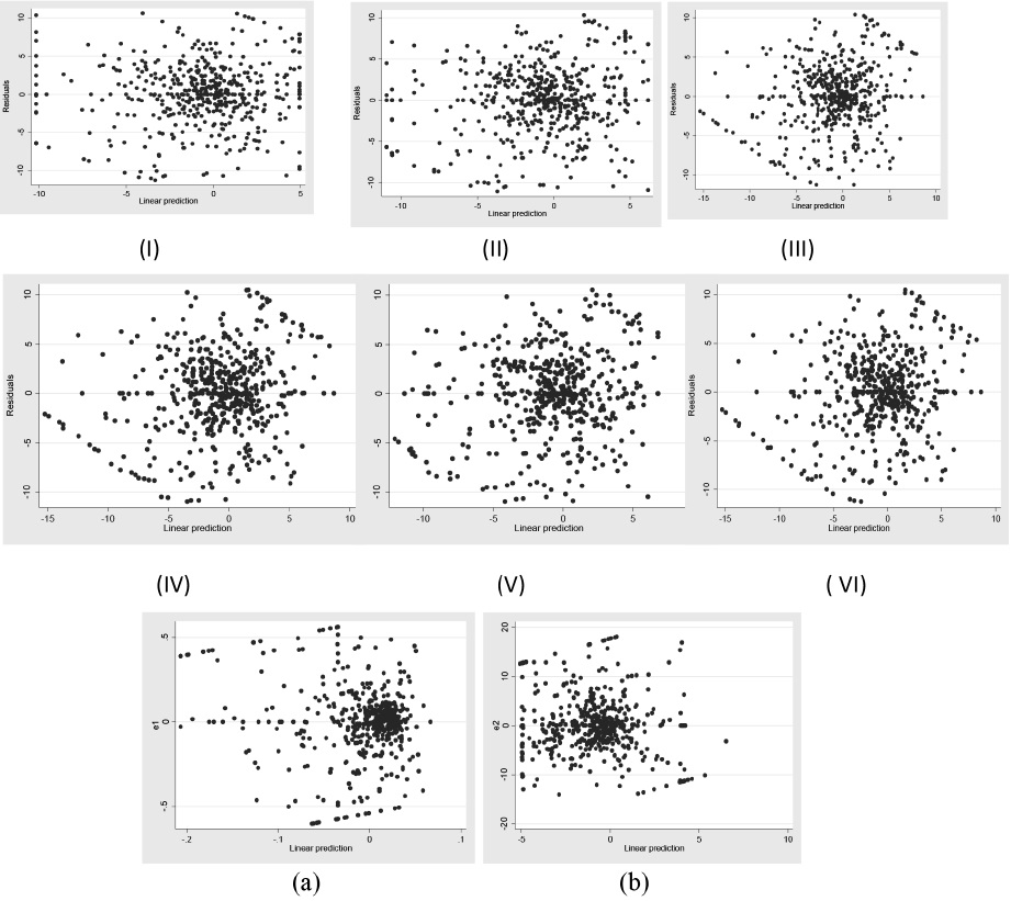
Source: Own elaboration
Figure 2 Scatterplot of the errors and estimated values of the dependent variable for each of the models (indicated in parenthesis).
Table 4 Model specification tests
| Models | ||||||||
|---|---|---|---|---|---|---|---|---|
| I | II | III | IV | V | VI | a | b | |
| Normaly test | ||||||||
| chi2(2) | 2.28 | 4.28 | 2.62 | 1.63 | 3.87 | 2.27 | 15.28 | 3.12 |
| P-value | 0.3197 | 0.1177 | 0.2701 | 0.4427 | 0.1441 | 0.3219 | 0.005 | 0.2097 |
| Heteroscedasticity test | ||||||||
| Breusch-Pagan /Cook-Weisberg | 1.390 | 0.090 | 0.020 | 0.010 | 0.020 | 0.040 | 33.07 | 2.310 |
| P-value | 0.239 | 0.767 | 0.893 | 0.925 | 0.879 | 0.842 | 0.000 | 0.129 |
| Serial correlation test | ||||||||
| Durbin-Watson | 1.851 | 1.837 | 1.813 | 1.866 | 1.794 | 1.843 | 1.828 | 1.874 |
| Critical value (DL) α=0.05 | 1.846 | 1.831 | 1.831 | 1.818 | 1.827 | 1.818 | 1.840 | 1.840 |
| Critical value (DU)- α=0.05 | 1.854 | 1.866 | 1.866 | 1.879 | 1.870 | 1.879 | 1.857 | 1.857 |
| Multicollinearity test - VIF | ||||||||
| RNOAt | 1 | 1.06 | 1.17 | 1.19 | 1.16 | 1.19 | ||
| CrNOAt | 1.18 | 1.18 | 2.07 | |||||
| ΔATOt | 1.13 | 1.91 | 1.93 | |||||
| ΔPMt | 1.15 | 2.00 | 1.12 | 1.14 | ||||
| Δ PM y ∇ ATO | 1.34 | 1.8 | ||||||
| ∇ PM y ∇ ATO | 1.37 | 1.94 | ||||||
| ∇ PM y ∇ ATO | 1.44 | 3.05 | ||||||
| Δ ATO y ∇ CrNOA | 1.59 | 2.29 | ||||||
| ∇ ATO y Δ CrNOA | 1.60 | 2.35 | ||||||
| ∇ ATO y ∇ CrNOA | 1.51 | 2.48 | ||||||
| ATO | 1.00 | |||||||
| Δ ATOt | 1.00 | |||||||
| PM | 1.17 | |||||||
| ΔPMt | 1.17 | |||||||
Source: Own elaboration.
The results plotted in Figure 2 and Table 4 were obtained for the different models by the classical MCO and the model specification results are as follows. The asymmetry and kurtosis test indicate a normal distribution of errors with the exception of model “a”, however, the corresponding scatterplot shows a distribution that is close to normal. The heteroscedasticity test shows that the assumption of equal variance for model “a” is not met. In the case of the non-autocorrelation scenario, the Durbin-Watson test indicates that, although most models are located in the area of uncertainty, with the exception of Models III, V and “a” in the rejection area and model “b” in the area of acceptance of the null hypothesis. The inflation factor of the variance (FIV) is much lower than 10, which indicates the absence of collinearity.
In financial studies, where panel data containing observations from multiple firms and multiple time periods are commonly used, the MCO estimate can produce residues correlated across firms and over time. The violation of the assumptions of homoscedasticity and nonserial correlation by MCO produces standard errors of the biased estimators that are crucial in the testing of the hypotheses. The problem is solved by the standard error method clustered by company and year (Thompson, 2011; Cameron, Gelbach and Miller, 2009). In this method the variance matrix of the MCO estimators is obtained from the sum of the estimated variance estimates grouped by company and time, minus the usual variance matrix of robust MCO variances to heteroscedasticity (Thompson, 2011). Peterson (2008) asserts that standard errors clustered by company and year are more suitable for the correction of residues than other methods used (White, Newey-West, Fama-MacBeth and fixed and random effects models). According to the method, the coefficients of the estimators are not modified if the variancecovariance matrix is modified.
The Voung test statistic is used to contrast the significance between the R 2 of two models that have the same dependent variables but different independent variables. A positive (negative) value indicates a better (worse) explanatory power of each of the models in relation to Model I, which is used as reference.
Discussion of the results
Table 5 shows the results obtained from the different models for predicting the change in the RNOA for the following year. In Model I, the coefficient of RNOAt is significant and indicates an inverse relationship with ∆RNOAt+1, by which the greater the value of current profitability, the lower the future profitability will be and vice versa. The coefficient obtained (β1=-0.390;t=-13.43) is much higher than the results obtained for the United States by Penman and Zhang (2002) (β1 =-0.176) and Fairfield and Yohn (2001) (β1=-0.1492), indicating a more pronounced process of mean reversion, which could be due to the context of instability.
Table 5 Results of the regression by model
| Models | ||||||
|---|---|---|---|---|---|---|
| Variables | I | II | III | IV | V | VI |
| Constant | 0.922 | 0.606 | 0.773 | 0.378 | 0.939 | 0.701 |
| 4.20 | 1.77 | 3.61 | 0.91 | 3.83 | 2.12 | |
| RNOAt | -0.390 | -0.394 | -0.341 | -0.344 | -0.370 | -0.340 |
| -13.43 | -15.62 | -12.31 | -12.59 | -13.33 | -15.18 | |
| CrNOAt | -0.054 | -0.059 | -0.066 | |||
| -3.80 | -4.21 | -4.04 | ||||
| ∆ATOt | 3.820 | 4.252 | 4.214 | |||
| 4.05 | 4.31 | 4.24 | ||||
| ∆PMt | -0.113 | -0.097 | -0.089 | -0.108 | ||
| -4.42 | -2.82 | -3.77 | -4.45 | |||
| PM increase and ATO decrease | -0.926 | 0.813 | ||||
| -0.55 | 1.27 | |||||
| PM decrease and ATO increase | 1.478 | 0.599 | ||||
| 3.19 | 0.81 | |||||
| PM decrease and ATO decrease | 0.009 | 0.604 | ||||
| 0.02 | 0.97 | |||||
| ATO increase and CrNOA decrease | 0.643 | -0.159 | ||||
| 1.58 | -0.30 | |||||
| ATO decrease and CrNOA increase | -1.149 | 0.420 | ||||
| -2.79 | 0.92 | |||||
| ATO decrease and CrNOA decrease | 0.210 | 0.223 | ||||
| 0.28 | 0.35 | |||||
| Adjusted R2 | 0.348 | 0.408 | 0.439 | 0.438 | 0.142 | 0.439 |
| Vuong Statistic | -1.474 | -1.960 | -1.991 | -1.494 | -2.038 | |
(*) The t-statistic is indicated below each coefficient, the coefficients in bold indicates that they are significant at 10%. Source: Own elaboration.
In Model II, the inclusion of the interaction between the signs (positive and negative) of margin changes and turnout does not show predictive power, the Vuong statistic is not significant. The coefficient of the current RNOA is significant and very similar in value to Model I. The RM2 coefficient (∆ATOt>0 and ∆PMt<0), significant and positive (β3=1.478; t=3.19), indicates a greater effect (∆ATOt>0 and ∆PMt>0) than that represented by the original ordinate, which in principle could be attributed to the earnings management effect, were it not for the fact that the opposite effect represented by RM1 (∆ATOt<0 and ∆PMt>0) is not significant. As a result, the increase in ATOt and PMt does not have a lasting effect over time, possibly due to the need to adjust expenses over time in the face of higher sales.
Model III exhibits greater explanatory power than Model I (Adjusted R2: from 0.4390 to 0.384), which is significant according to the Vuong statistic, due to the additional effect of Dupont disaggregation. The coefficients are all significant, the coefficients for CrNOAt (β2=-0.054; t=-3.80) and ∆PMt (β4=-0.113; t=-4.42) are negative and for ∆ATOt (β3=3.820; t=4.05) it is positive, with regard to ∆RNOAt+1. In short, the only variable that predicts a sustainable increase in future profitability is the increase in ∆ATOt, which is consistent with different studies, while ∆PMt has a negative effect, according to the study by Bauman (2014), but not according to Fairfield and Yohn (2001). In Model IV, the coefficients that capture the interaction between the signs of margin change and turnover coefficients are not significant, therefore, this model does not provide relevant information in relation to Model I, according to the Vuong statistic.
Model V exhibits greater explanatory power than Model I, but according to the Vuong statistic it is not significant. The results show a negative effect of the coefficients RNOAt(β1=-0.370; t=-13.33) and ∆PMt, (β2=-0.089; t=-3.77). The variable GR1 that represents (∆ATOt<0 and CrNOAt>0) is negative and significant (β4=-1.149; t=-2.79) in relation to the positive and significant source ordinate (α=0.939; t=3.83) that reflects (∆ATOt>0 and CrNOAt>0). This indicates that the greatest effect corresponds to (∆ATOt>0 and CrNOAt>0) and is the case where new investments produce an increase in sales. The coefficients of variables GR2 and GR3, although positive, are not significant.
Finally, Model VI adds the interaction between ∆ATOt and CrNOAt and to model III. The aggregate variables do not have a significant effect on ∆RNOAt+1, therefore, the results are similar to Model III, in terms of the explanatory power and significance of the coefficients.
Table 6 shows the results obtained from the models for the prediction of the change in PM and ATO for the following year. A first consideration is that in both models, the coefficients of ATOt (β1=-0.057; t=-3.38) and PMt (β1=-0.157; t=-4.24) are significant and negative, thus the reversal process of the RNOA is produced by both the reversal of ATOt and PMt. On the other hand, ∆ATOt exhibits a positive and significant effect (β2=0.298; t=4.52) on ∆ATOt+1, and ∆PMt exhibits a negative and significant effect (β_3=-0.295; t=-6.79) on [text missing] and ∆PMt+1. This confirms the positive effect of the change in turnout and the negative effect of the change in the profit margin on the profitability of the following year.
Conclusions
The aim of this work is to assess the short-term predictability of current return on net operating assets and the change in the profit margin and turnover of current net operating assets. The calculation of profitability is determined by the permanent components of the results. From the discussion of the different models proposed for the prediction of the change in the RNOA of the following year, the following conclusions emerge:
In the previous analysis, at an aggregate level, the trend of the annual mean turnover shows a more stable behavior of the turnover than the margin, being affected mainly by the level of activity.
The change in the profit margin and asset turnover shows additional predictive power over and above current profitability.
The RNOA of the following year shows a strong reversal with respect to the current RNOA, it is even higher than in other similar studies in developed countries. This is produced by the reversal of the turnover of assets and the profit margin.
The growth in net operating assets shows a negative effect on the RNOA of the following year, which is likely due to conservative accounting criteria.
The earnings management effect, controlled through the ATO-PM ratio, showed no relevant effect, which is quite logical considering that the items that comprise the results analyzed are those that make up the main operating activity.
The combined effect of a decrease in the profit margin and an increase in turnover has a greater effect on the RNOA of the following year than the increase in both. This is consistent with the fact that the change in profit margin is not persistent in time.
The change in the turnover of assets has a positive effect on the change in the RNOA of the following year, with efficiency allowing for an improvement in profitability. In turn, individually, the change in turnover shows a positive effect on the change in the turnover of the following year.
The increase in the profit margin reverses rapidly, with a negative effect on the RNOA of the following year and shows a negative effect on the change of the profit margin of the following year.
REFERENCES
Aguiar, M y Gopinath, G. (2007). Emerging market business cycles: The cycle is the trend. Journal of Political Economy 115: 69-102. http://dx.doi.org/10.1086/511283 [ Links ]
Amir, E, Kama, I y Levi, S. (2015). Conditional Persistence of Earnings Components and Accounting Anomalies. Journal of Business Finance & Accounting, 42, 801-825. http://dx.doi:10.1111/jbfa.12127 [ Links ]
Anuarios del Instituto Argentino del Mercado de Capitales-IAMC (2002-2012). Disponible en http://www.iamc.sba.com.ar/informes/informe_anuario/ . Consultado: 30/04/2014. [ Links ]
Arbanell, J S y Bushee B J. (1997). Fundamental analysis, future earnings, and stock prices. Journal of Accounting Research, 35, 1-24. http://dx.doi.org/10.2307/249 1464 [ Links ]
Bauman, M P. (2014). Forecasting operating profitability with DuPont analysis. Review of Accounting and Finance, 13(2), 191-205. http://dx.doi:10.1108/raf-11-2012-0115. [ Links ]
Canarella, G; Miller, S M y Nourayi, M M. (2013). Firm profitability: Mean-reverting or random-walk behavior? Journal of Economics and Business, 66, 76-97. http://dx.doi.org/10.1016/j.jeconbus.2012.11.002 [ Links ]
Cameron, A C, Gelbach, J, y Miller, D L. (2009). Robust Inference with Multiway Clustering. NBER Technical Working Paper Number 327. https://doi.org/10.3386/t0327 [ Links ]
Esplin, A, Hewitt, M , Plumlee, M y Yohn, T L. (2013). Disaggregating operating and financing activities. Implications for forecasts of future profitability. Review of Accounting Studies, 19, 328-362. https://doi.org/10.1007/s11142-013-9256-5 [ Links ]
Fama, E F y French K R. (2000). Forecasting Profitability and Earnings. The Journal of Business, 73(2), 161-175. https://doi.org/10.1086/209638 [ Links ]
Fairfield, P., R Sweeneyy T. Yohn, T L. (1996). Accounting Classification and the predictive Content of Earnings. The Accounting Review, 71, 337-355. Obtenido de https://www.jstor.org/stable/248292 . Consultado: 01/07/2015. [ Links ]
Farfield, P M y Yohn T L. (2001). Using asset turnover and profit margin to forecast changes in profitability. Review of Accounting Studies, 6, 371-385. https://doi.org/10.1023/a:1012430513430 [ Links ]
Fondo Monetario Internacional (2013). Perspectivas Políticas Mundiales-octubre 2013. Disponible en http://www.imf.org/external/spanish/pubs/ft/weo/2013/02/pdf/texts.pdf , Consultado: 18/10/2013. [ Links ]
Hejazi, R., Adampira, S., Bahrami, Z M. (2016). A Diagnostic for Earning Management by Using Changes in Asset Turnover and Profit Margin. The Financial Accounting and Auditing Researches, 8 (29), 73-95. Obtenido de http://www.sid.ir/En/Journal/ViewPaper.aspx?ID=483292 . Consultado: 01/07/2016. [ Links ]
Jansen, I, Ramnath, S y Yohn, T L. (2011). A diagnostic for earnings management using changes in asset turnover and profit margin. Contemporary Accounting Research, 29 (1), 221-251. https://doi.org/10.1111/j.1911-3846.2011.01093.x [ Links ]
Konchitchki, Y. (2011). Inflation and Nominal Financial Reporting: Implications for Performance and Stock Prices. The Accounting Review 86(3), 1045-1085. http://dx.doi.org/10.2308/accr.00000044 [ Links ]
Lev, B. y Thiagarajan S. (1993). Fundamental information analysis. Journal of Accounting Research 31: 190-215. http://dx.doi.org/10.2307/2491270 [ Links ]
Lipe, R y Kormendi, R. (1994). Mean Reversion in Annual Earnings and Its Implications for Security Valuation. Review of Quantitative Finance and Accounting 4: 24-46. http://dx.doi.org/10.1007/BF01082663 [ Links ]
Mahmud, R, Ibrahim, M K, y Pok, W C. (2009). Earnings Quality Attributes and Performance of Malaysian Public Listed Firms. http://dx.doi.org/10.2139 /ssrn.1460309 [ Links ]
Missim D y Penman, S H. (2001). Ratio Analysis and Equity Valuation: From research to practice. Review of Accounting Studies, 6,109-154. https://doi.org/10.1023/A1011338221623 [ Links ]
Monterrey, J y Sánchez-Segura, A. (2011). Persistencia y capacidad predictiva de márgenes y rotaciones: un análisis empírico. Revista de Contabilidad-Spanish Accounting Review, 14(1), 121-153. https://doi.org/10.1016/S1138-4891(11)70024-3 [ Links ]
Monterrey Mayoral, J y Sánchez Segura, A (2017). Una evaluación empírica de los métodos de predicción de la rentabilidad y su relación con las características corporativas. Revista de Contabilidad-Spanish Accounting Review, 20(1), 95-106. http://dx.doi.org/10.1016jrcsar.2016.08.001. [ Links ]
Mueller, D C. (1977). The Persistence of Profits above the Norm. Economica, 44(176), 369-380. https://doi.org/10.2307/2553570 [ Links ]
Notz, S y Rosenkranz, P. (2014). Business cycles in emerging markets: the role of liability dollarization and valuation effects. Working paper Nº 163 University of Zurich. https://doi.org/10.2139/ssrn.2459001 [ Links ]
Ohlson, J. (1995). Earnings, book values, and dividends in equity valuation. Contemporary Accounting Research, 22(2), 661-687. https://doi.org/10.1111/j.1911-3846.1995.tb00461.x [ Links ]
Ou, JA. (1990). The information content of nonearnings accounting numbers as earnings predictors. Journal of Accounting Research, 28, 144-163. http://dx.doi.org/10.2307/2491220 [ Links ]
Penman, S H y Zhang X. (2002). Modeling sustainable earnings and P/E ratios with financial statement analysis. Working paper de la Columbia University y University of California, Berkeley. http://dx.doi.org/10.2139/ssrn.318967 [ Links ]
Petersen, M A. (2009). Estimating standard errors in finance panel data sets: Comparing approaches. Review of financial studies, 22(1), 435-480. http://dx.doi.org/10.1093/rfs/hhn053 [ Links ]
Richardson, S, Tuna, I y Wysocki, P (2010). Accounting anomalies and fundamental analysis: A review of recent research advances. Journal of accounting & economics, 50(2-3 ), 410-454. http://dx.doi.org/10.1016/j.jacceco.2010.09.008 [ Links ]
Sandin, A y Porporato, M. (2007). Corporate bankruptcy prediction models applied to emerging economies. Evidence from Argentina in the years 1991-1998. International Journal of Commerce and Management, 17(4), 295-311. http://dx.doi.org/10.1108/1056921071084437. [ Links ]
Selling, T I y Stickney, C. (1989). The effects of Business Environment and Strategy on a Firm´s Rate of Return on Assets. Financial Analysts Journal, 45(1), 43-68. https://doi.org/10.2469/faj.v45.n1.43 [ Links ]
Soliman, M T. (2004). Using Industry-Ajusted DuPont Analysis to Predict Future Profitability. Working Paper Working Paper Stanford University. http://dx.doi.org/10.2139/ssrn.456700. [ Links ]
Stigler, G. (1963). Capital and Rates of Return in Manufacturing Industries. Princeton, NJ: Princeton University Press. [ Links ]
Swanson, E P, Rees, L y Juárez-Valdés, L F. (2003). The contribution of fundamental analysis after a currency devaluation. The Accounting Review, 78(3), 875-902. https://doi.org/10.2308/accr.2003.78.3.875 [ Links ]
Tabachnick, B G y Fidell, L S. (2001). Using Multivariate Statistics (4th Ed). New York: Allyn & Bacon. [ Links ]
The Economist (2013). When giants slow down. Disponible en http://www.economist.com/news/briefing/21582257-most-dramatic-and-disruptive-period-emerging-market-growth-world-has-ever-seen . Consultado: 20/11/2014. [ Links ]
Thompson, S B. (2011). Simple formulas for standard errors that cluster by both firm and time. Journal of financial Economics, 99(1), 1-10. http://dx.doi.org/10.1016/j.jfineco.2010.08.016 [ Links ]
Zanjirdar, M., Khaleghi Kasbi P. y Madahi Z. (2014). Investigating the effect of adjusted DuPont ratio and its components on investor’s decisions in short and long term- Management Science Letters, 4,591-596. http://dx.doi.org/10.5267/j.msl.2014.1.003 [ Links ]
3NCPs: accounting standards issued by the Argentinian Federation of Professional Council of Economic Sciences (FACPCE for its acronym in Spanish).
4This same index is used by the Argentinian Institute of Capital Markets (IAMC for its acronym in Spanish) for the adjustment of its data.
Received: July 05, 2016; Accepted: December 05, 2017
 Este es un artículo publicado en acceso abierto bajo una licencia Creative Commons
