Introduction

The α-stable distributions are a more adequate alternative to model financial series that show clusters of high volatility, extreme values that present a greater frequency than expected due to the Gaussian distribution, and that have a greater financial and economic impact with respect to the probable income statements derived from the yields, complying with the generalized central limit theorem. Therefore, the yields are in the attraction domain of an α-stable law, where the Gaussian distribution is a particular case that cannot adequately model the extreme values and the asymmetry of the financial and economic series. Thus, the α-stable distributions allow the proper estimation of the confidence levels for the financial engineering and risk administration projects through the appraisal of derived products, structured products, value at risk, and conditional value at risk, utilizing the relation between the self-similar exponent and the stability parameter.

^{Panas (2001)} indicates that the α parameter represents the fractal dimension of the probability space. The relation between this dimension and the fractal dimension of the time series is expressed by the self-similar exponent H=α^-1 , while the fractal dimension of the time series is D=2-H. The H exponent is related to the effects of persistency, concluding that when α ^-1 ≤H<1, the series is persistent or presents a long-term memory; and when 0<H< α^-1, the series is anti-persistent or presents a short-term memory. It indicates that the α-stable distributions are utilized to estimate the shapes of the distributions and the fractal dimensions. The rescaled range analysis (RR) provides a relation between the H exponent and the a parameter, where H= α ^-1 . The applications are based on the α stability parameter and are valid only if the yields have an α-stable distribution. Furthermore, the author analyzes the Athens Stock Exchange and thirteen analyzed yields (100%) reject the Gaussian distribution hypothesis, 11 out of 13 yields (84.62%) present α-stable distributions, and 11 stability parameters (100%) are H>2^-1, providing evidence of persistence in the Athens Stock Exchange.

^{Muñoz San Miguel (2002)} defines the self-similar exponent as H-as, where H>0. He indicates that the Brownian motion (Bm) is self-similar with exponent H=2^-1, the Fractional Brownian Motion (fBm) is H-as with 0<H< 1, persistent when 2^-1<H<1, and anti-persistent when 0<H<2^-1. He defines the Lévy processes and indicates that the α-stable processes are the only Lévy processes H-as. Munoz also estimates the fractal dimension of the time series of the Spanish index IBEX35 as D=1.3663±0.0202 through the box counting method (BCM). He indicates that the fBm has a fractal dimension D=2-H. The α-stable movement (MS) is a stochastic process H-as with the exponent H=α ^-1 and has a finite expectation, that is, if 1<α≤2 has a fractal dimension D=2-α ^-1 , then the self-similar exponent of the IBEX35 is H=2-D=0.6337±0.0202 and the stability parameter is α=(2-D)^-1=1.5780±0.0520. He concludes that the IBEX35 can be modeled with an H-as process combining the fBm with an α-stable process.

^{Samorodnitsky (2004)} asks how to decide if a symmetric and stationary α-stable process presents a long-term dependence. He indicates that the random α-stable variables where 0<α<2 have a second non-finite moment, and that the correlations to indicate if a stationary α-stable process presents long-term dependence cannot be used. The family of Gaussian processes is the fBm, the self-similar exponent is 0<H<1, the partial sums of the increments of the process increase at a rate greater than n2-1 when H>2^-1, therefore, the quota between the short- and long-term memory for the fBm is H=2^-1. The stationary increments of the α-stable processes H-as, when 1<α< 2, have a non-finite variance and a 0<H<1 exponent. The limit of the partial sums of the increments increase at a rate greater than the independent distributions and which are identically distributed, that is, faster than n2-1 , which is the case H=2^-1. He concludes that the H=2^-1 quota is not possible for α-stable processes H-as with stationary increments when 0<α<1, and that long-term dependence is not possible when 0<α<1.

^{Belov, Kabašinskas, and Sakalauskas (2006)} indicate that the α-stable processes must justify their suitability in the market and that they have become a potent and versatile tool in financial models. They demonstrate the adequacy and efficiency of the α-stable parameters estimated by the maximum likelihood estimation. They also carry out hypothesis tests for multifractality and for self-similarity, and present an analysis for the Hurst exponent. They indicate that there are two reasons as to why the α-stable paradigm is applied to financial processes: the first is that the random α-stable variables justify the generalized central limit theorem, establishing that the α-stable distributions are the only asymptotic distributions that are adequate for the sum of random escalated, central, independent and identically distributed variables; the second is that they are leptokurtic and asymmetrical. From the point of view of financial engineering, the α-stable distributions must be applied to the financial portfolios because the diversification of resources is also α-stable. The maximum likelihood method provides the best results to estimate the parameters because it is the most precise. Hypothesis tests for the Gaussian distribution were carried out and the Anderson-Darling (AD) statistics were utilized for the α-stable distributions, as they are more sensitive in the extremes of the distribution; while Kolmogorov-Smirnov (KS) was also utilized, being more sensitive in the central part of the distribution. The Gaussian distribution hypothesis of 27 yields is rejected (100%) through the AD statistic, and the α-stable distribution hypothesis of 15 out of 27 yields (55.56%) with a significance level of 5% is also rejected. The authors conclude that the convenient models are the non-Gaussian with Pareto properties because they adequately model the leptokurtosis and asymmetry of the yields; they also indicate that the stability test can be carried out through the variance convergence, homogeneity, self-similarity, and multifractality methods using the Hurst exponent to characterize the fractal dimension. When 0<H<2^-1, the processes present a mean reversion, if X(t) is a Lévy process, then X(t) is H - as if and only if X(t) is strictly α-stable and the H=α ^-1 relation is satisfied. To estimate the Hurst exponent in the time domain, they utilize the absolute moments (AM), variance convergence (VC), rescaled range (RR) and residual variance (RV) methods, and in the frequency domain they utilize the periodogram (PG), and Whittle and Abry-Veitch (WAV) methods. They conclude that the α-stable models are adequate for financial engineering, but only 22% of the yields are α-stable, therefore, it is necessary to adapt the model and other stability tests.

^{Luengas Domínguez, Ardila Romero, and Moreno Trujillo (2010)} indicate that the markets are not always Gaussian, complete, efficient and free of adjudication; the yields are not stationary - they have a long- or short-term dependence and leptokurtosis-, therefore, the Bm is not an adequate representation of reality. The GARCH models do not represent the long-term dependence, they define the fBm where the Hurst exponent is the independence measure in order to distinguish fractal series when 0<H<1, with a cyclical and non-periodic variance in all time scales. They indicate that a non-parametric RR analysis is used in order to distinguish the fractal series and they describe the methodology for the estimation of the exponent and its characteristics, indicating that 0<H<1 is unique, and that if 0<H<2^-1 the correlation is negative and the series are anti-persistent or present mean reversion, if H=2^-1 the correlation is null and the series are independent; and if 2^-1<H<1, the correlation is positive and the series are persistent. Furthermore, the authors define the fractal dimension based on the Hurst exponent as D=2-H, utilizing the CR method for the estimation of the exponent; they estimate the exponent for five Colombian series. They conclude that it is advisable to estimate the Hurst coefficient to prove the independence assumption.

^{Barunik and Kristoufek (2010)} show that the properties in the estimation of the Hurst exponent change with the presence of leptokurtosis. They carry out Monte Carlo simulations to understand how the RR analysis, multifractal detrended fluctuation analysis (MFDFA), the detrended moving average (DMA), and the generalized Hurst exponent (EHG). They also estimate the Hurst exponent from independent series with different stability parameters; they indicate that the EHG method provides the lowest variance and bias with regard to the other methods; they estimate the Hurst exponent with high frequency data (per second); they present results for independent α-stable processes and study the sampling properties with leptokurtosis; they estimate expected values and confidence intervals for RR, MFDFA, DMA and EHG with series of 2⁹ and up to 2¹⁶ observations; they indicate that the MFDFA is a generalization of the detrended fluctuation analysis (DFA) and allow using multifractal and non-stationary data. They also indicate that it has been demonstrated that the EHG is H(q)≈q ^-1 , so that q>α, and that H(q)≈α ^-1 for q≤α. The DMA method is based on the deviations of the moving average of the full time series. The EHG method is adequate for multifractal detection, since it is based on the scale of q order moments for the increments of X(t). The statistical scale is K _q (τ)≈cτ ^qH(q) and is comparable with the estimators of RR, DMA and MFDFA(2). When q=1, H(1) is characterizing the scale of the absolute deviations of the process; RR overestimates the Hurst exponent and DMA underestimates it; RR and DFA are robust for different distributions and both are sensitive to the presence of short-term dependence; VR presents the relation E(H)≠2^-1 and E(H)=α^-1 for independent α-stable processes, which is equal for MFDFA(1) when 1≤α≤2. The authors also indicate that the generalization of DFA with the MFDFA(q) with the theoretical H(q)≈q ^-1 for q>α and H(q)≈ α^-1 for q≤α has been proposed. The properties for the finite samples of the DFA and the DMA are compared for the standard Gaussian process, and the DFA surpasses the DMA in matters of bias and variance, noting that the results are questionable because the estimations only consider the cases with R ² > 0.98. Furthermore, the estimation of the Hurst exponent is done without any discussion regarding the omitted estimations and the selection of the lags is not discussed for the DMA method. The efficiency of RR is examined with contiguous and superimposed sub-series, and the methods do not significantly differ; RR and DFA show that the bias and the average of the square errors are lower for RR than for DFA. The behavior of RR, DFA, MFDFA, DMA and EHG with independent and equally distributed α-stable series when 1.1≤α≤2 depends on the α parameter; the expected value of RR converges to 2^-1 with the presence of more leptokurtosis; the DMA method has similar properties but it is more precise; the DFA method is less precise than RR and DMA; the MFDFA(1) presents E(H)=α^-1 and E(H)≠2^-1 but underestimates the real value, whereas the MFDFA(2) is equivalent to the DFA; the EHG(1) and MFDFA(1) methods present E(H)=α^-1, therefore, EHG(1) presents the best behavior for finite samples among all the methods, with the lowest variance, lowest bias and the narrowest confidence intervals; RR and EHG(2) are robust with more leptokurtosis; DMA, DFA and MFDFA(1) deteriorate with the presence of more leptokurtosis, but they surpass the estimation of RR for Gaussian series, that is, when α=2. The situation changes for non-Gaussian simulations; the MFDFA(1) tends to underestimate E(H)=α^-1; the MFDFA and DMA are not appropriate for the series with greater leptokurtosis and smaller-sized samples. They conclude that RR and EHG are robust, the EHG(q) surpass all the other methods; DMA, DFA and MFDFA(q) tend to deteriorate with the increase of leptokurtosis, whereas with Gaussian series all the methods present the expected 2^-1 value and, therefore, seem to be better than RR for the estimation of the self-similar exponent. The situation changes with non-Gaussian series: when the series present a greater leptokurtosis, the confidence intervals are broader; the MFDFA(1) tends to underestimate E(H)=α^-1, the MFDFA(q) and DMA are not appropriate for the series with greater leptokurtosis nor for smaller-sized samples, therefore, the EHG(q) methods proved to be useful given that they show the best properties.

^{Quintero Delgado and Ruiz Delgado (2011)} present an alternative to estimate the Hurst exponent through the RR analysis and the fractal dimension, where the Hurst exponent is an independence measure of the time series. When H=2^-1, there are random and independent processes that present a null correlation between the increments; when 2^-1<H<1, there are persistent processes, which are positively correlated and have long-term memory; when 0<H<2^-1, there are anti-persistent processes, which are negatively correlated and have short-term memory. They conclude that the processes of the topographic profiles are persistent.

^{Rodríguez Aguilar (2014)} addresses the usefulness of the estimation of the stability parameter of the α-stable distributions and the Hurst coefficient in high volatility periods to explore the abuse of a priori Gaussian distribution and independence assumptions, identifying fractal and leptokurtic characteristics in the parity of the FIX exchange rate. He also finds five sub-periods of high volatility and calculates the Hurst exponent and the stability parameter to verify if the assumed Gaussian and independence are simultaneously being infringed upon. He builds an index to evaluate the distance of the independence and Gaussian distribution assumptions. He describes the RR method and estimates the Hurst exponent for transversal cuts in high volatility periods and rejects the independence hypothesis in 4 of the 5 periods (80%). He estimates the stability parameter and finds consistency with the Hurst exponent. He concludes that progress is made for the improvement of the modeling of financial series through the index.

^{Salazar Núnez and Venegas-Martínez (2015)} examine the dynamic of the exchange rate of the American dollar for several economies utilizing the Hurst exponent, correlogram, variance graph, and the local Whittle and Robinson estimation. They indicate that Chile, China, Iceland, Israel, Mexico and Turkey present evidence of long-term memory, therefore, they estimate an Autoregressive fractionally integrated moving average (ARFIMA) in the time and frequency domains. In the time domain, the maximum likelihood estimation was utilized, while in the frequency domain, the Fox and Taqqu technique was used. The results of the ARFIMA model show that Chile, China, Iceland and Mexico present evidence of long-term memory. The method that presents the best fit is the exact maximum likelihood method, in accordance with the Akaike information criterion. They concluded that the correlogram tests, variance graph, and Hurst coefficient indicate that there is long-term memory with the exception of South Korea and Indonesia through the variance graph method, and with Chile and Israel through the Hurst exponent.

The objective of this research work is to estimate the (α, H) pair to know the α-stable distributions, the fractal dimensions of the probability spaces (Ω, ℱ, ℘), the fractal dimensions of the time series, the anti-persistence, independence or persistence effects and the movements (ME, MELF or MElogF) with which it is possible to adequately model the time series of the parities of the FIX, Euro, Yen and Canadian dollar exchange rates that depend on the (α, H) pair relation. Using the maximum likelihood estimation to estimate the parameters of the α-stable distributions, as well as the EGH(1) method to estimate the exponents of self-similarity H and to estimate confidence intervals for the distributions of the parities of the types of exchange and compare them to the Gaussian confidence intervals, future works can appraise derived financial products, structured products and value at risk through the estimated distributions, the anti-persistence, independence or persistence effects.

The work is organized in the following manner: the second section presents the definitions and more relevant properties of the α-stable distributions, as well as the relation between the stability parameter and the self-similar exponent that indicate if the process is anti-persistent, independent or persistent; the third section presents the analysis of the parity yields of the exchange rates, the estimation of the basic statistics, the estimation of the α-stable parameters, the goodness of fit tests, and the estimation of the self-similar exponents; in the fourth section we carry out the estimation of the confidence intervals of the parities of the exchange rates; and in the fifth section we present the conclusions of the research work and the bibliography.

The α-stable distributions and the self-similar exponent

The self-similarity processes are invariant in distribution under the time and space scale. The self-similar α-stable distributions allow a greater variability that could show the effects with extended periods of abundance, extended periods of shortage, and with exceptional events of abundance and shortage.

The X(t) process is self-similar to the H>0 exponent, if for every α ϵ (0, ꝏ) the finite-dimensional distributions of X(at) are identical to the finite-dimensional distributions of a ^H X(t):

(1)

The symmetric α-stable Lévy movement (SLM) is H-as with H=α^-1, so that H ϵ [2^-1, ꝏ), that is, the Bm is H-as with H=2^-1.

If the X(t) process is H-as, then for every t ϵ ℝ the Y(t)=exp(-tH)X(exp(t)) process is stationary, and for every t ϵ (0, ꝏ) the X(t) = t ^H X(exp(ln(t))) process is H-as. If X(t) is the Bm, then Y(t)=exp(-2^-1 t)X(exp(t)) is an Orstein-Unlenbeck process.

The X(t) process has stationary increments for all t ϵ (0, ꝏ) when:

(2)

The X(t) process is H-asie, if it is self-similar and presents stationary increments. The SLM is a H-asie process with H=α^-1.

If the X(t) process is H-asie and ℘(X(1)≠0)>0, then E(|X(1)| ^p )<ꝏ, and therefore H ϵ (0, p ^-1 ) is satisfied when p ϵ (0, 1) and H ϵ (0, 1] when p ϵ [1, 2]. Figure 1 shows the region of values for the (α, H) pair.

Source: Own elaboration in a spreadsheet.

Figure 1 Region of values for the (α, H) pair. 

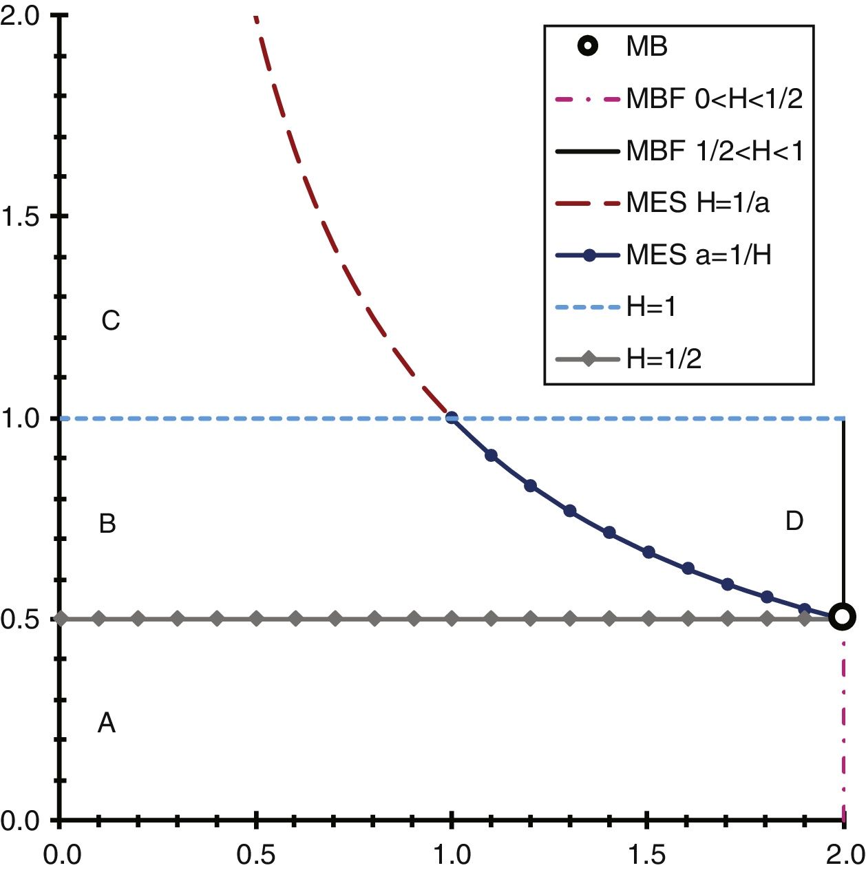
Figure 1 shows that the horizontal axis represents the values of parameter α and the vertical axis represents the values of exponent H, and regions A, B, C and D can be seen; the Bm is represented by the black circumference with the (2, 2^-1) pair, which indicates that the Bm is a particular case of the α-stable distributions. The fBm is represented by the vertical lines (pink dotted line for 0<H<2^-1 and a solid black line for 2^-1<H<1 for the (2, H) pair with H ϵ (0, 1), where the Bm is a particular case of the fBm with H=2^-1 and this is also a particular case of the α-stable distributions; the SLM is represented by the purple dotted line for H>1 and a solid navy blue line for H ϵ [2^-1, 1], which is obtained from the H= α^-1 relation for the α ϵ (0, 2] parameter; the linear fractional α-stable motion (MELF) is represented by the following sets:

where the sets A, B and C are anti-persistent processes and set D represents persistent processes; the ME is represented by the following sets:

where sets E (purple dotted line) and F (navy blue solid line) represent independent processes, and include the SLM and the Bm where this is a particular case of the SLM; the log-fractional α-stable motion (MElogF) is represented by the following set:

where set G (navy blue solid line) represents persistent processes for every α ϵ (1,2) parameter, the Bm is a process with independent increments and is also a particular case of the MElogF.

The fBm is a Gaussian H-asie process with H ϵ (0, 1) as well as a particular case of the α-stable distributions. The Bm is a particular case of the fBm when H=2^-1. The fBm is a particular case of sets A, D, F and G, that is, the fBm presents anti-persistent (set A), independent (sets D and F) and persistent (sets D, F and G) increments and is a particular case of the MELF, ME, SLM and MElogF. The Bm presents independent increments and is a particular case of sets F and G, that is, the Bm is a particular case of the ME, SLM and MElogF and also of the fBm.

The MELF is H-asie and is the most commonly used stochastic process where we have the α ϵ (0, 2] parameter, the H ϵ (0, 1) exponent and H≠α ^-1 . The fBm is a particular case of the MELF and also of the SLM when the asymmetry parameter is β=0. The MELF presents persistent increments when H>α ^-1 , set D; presents anti-persistent increments when H<α^-1 , sets A, B and C. If the X(t) process is a MELF, then for every fixed t ϵ ℝ, X(t) presents an α-stable distribution S(α, β _t , γ _t , δ _t ).

A ME is an X(t) process with stationary and independent increments with a strict α-stable distribution for every t ϵ (0, ꝏ). The Bm is a particular case of the ME with α=2. The ME is H-asie with the H=a ^-1 exponent, where H ϵ (2^-1, 2). The only α ^-1 -asie non-degenerate processes where the α ϵ (0, 1) parameter are the ME. When α ϵ (1,2], there is the MElogF that is also α^-1-asie.

With α ϵ (1, 2], X(t) as a stochastic process with stationary increments and M as a random α-stable measure on the set of ℝ real numbers, with a Lebesgue control measure and a β asymmetry parameter, a constant defines the MElogF. The MElogF is not defined for α≤1 because x ^-α is not integrable when x→ ꝏ. The MElogF is H-asie with H=α^-1 , and the Bm is a particular case of the MElogF with H=2^-1. The MElogF shows anti-persistent or persistent increments when α ϵ (1, 2), therefore, MElogF ≠ ME.

Analysis of the exchange rate parities

The exchange rate parities analyzed in this research are the American dollar (USD), the Canadian dollar (CAD), the Euro and the Yen, which are published by the Bank of Mexico, utilizing data from the period between 08-30-2007 (USD), 05-25-2007 (CAD), 08-28-2007 (EUR) and 0827-2007 (JPY) to 10-22-2015, with 2049 parities and 2048 yields. The analysis includes the basic statistics, the estimation of the α-stable parameters through the maximum likelihood method, the KS and AD tests to prove the distribution hypothesis, the estimation of the self-similar exponent through the EHG(1) method to know - through the relation between the stability parameter and the self-similar exponent - if the process presents anti-persistence, independence or persistence.

Figure 2 presents the USD, CAD, EUR, and JPY exchange rates with 2049 observations, where the exchange rate parity of the Yen represents one hundred Yen.

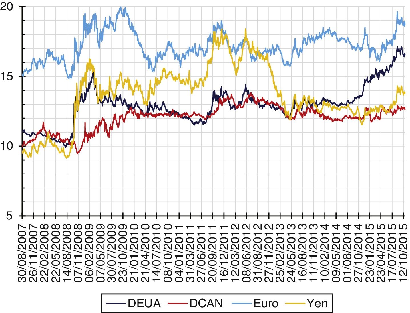
Source: Own elaboration in a spreadsheet with data from the Bank of Mexico.

Figure 2 Performance of the exchange rate parities. 

Estimation of the basic statistics of the yields

The period to estimate the α-stable parameters of the distributions of the yields of the exchange rate parities is from 08-30-2007 (USD), 05-25-2007 (CAD), 08-28-2007 (EUR) and 08-27-2007 (JPY) to 10-22-2015 with 2048 observations. The daily yields of the exchange rate parities are presented in Figure 2.

Figure 3 shows the performance of the daily yields of the exchange rate parities that present a minimum of -5.5975% and a maximum of 7.3328% for the USD, a minimum of -8.2157% and a maximum of 6.5427% for the CAD, a minimum of -5.5977% and a maximum of 7.5902% for the EUR, and a minimum of -5.8147% and a maximum of 9.6074% for the Yen. The yields present high volatility clusters that represent financial crises during short terms and lower volatility clusters that represent financial stability during longer terms than the crisis periods; these stylized events show the presence of bias and leptokurtosis in the distributions of the studied yields. The estimation of the basic statistics of the exchange rate parity yields are presented in Table 1.

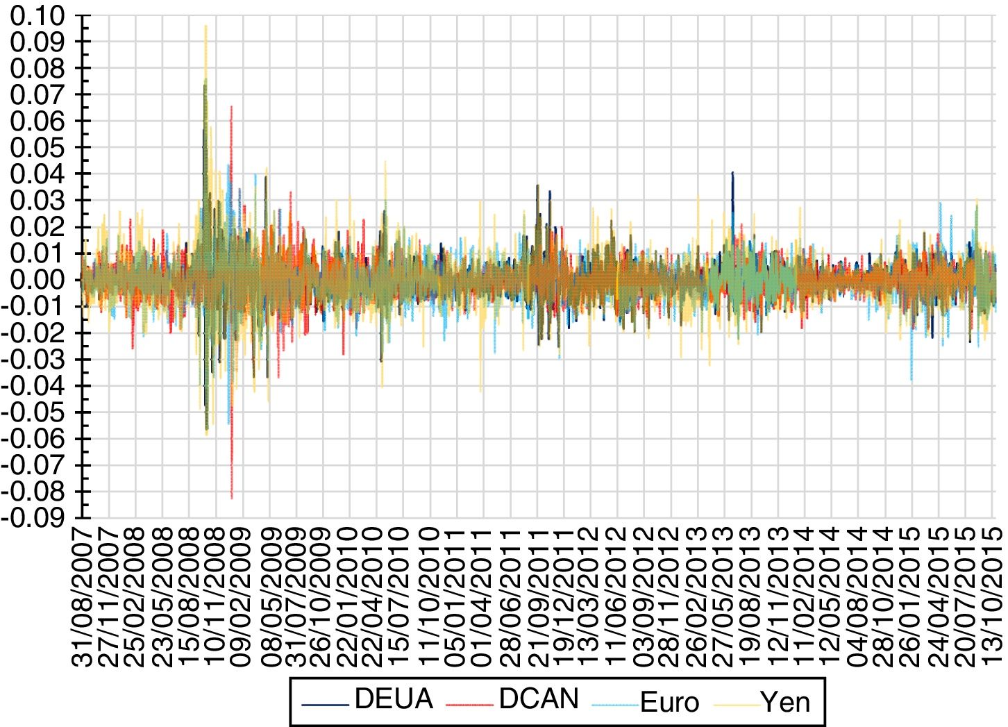
Source: Own elaboration in a spreadsheet with data from the Bank of Mexico.

Figure 3 Performance of the yields of the parities. 

Table 1 Basic statistics of the yields. 

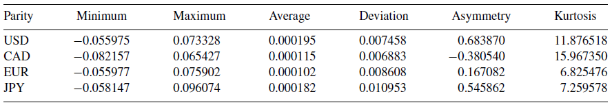
Source: Own elaboration in a spreadsheet with data from the Bank of Mexico.

Table 1 shows the basic statistics of the exchange rate parity yields: the averages indicate that the yields are appreciated with respect to the Mexican peso; the positive asymmetry coefficients indicate that the yields of the USD, EUR and JPY exchange rate parities present distributions that extend toward positive values with more frequency than they do toward negative values, and the negative asymmetry coefficient indicates that the CAD yields present a distribution that extends toward negative values with a higher frequency than they do toward positive values. The coefficients of kurtosis indicate that the distributions of the yields are leptokurtic with respect to the Gaussian distribution, concluding that the yields of the exchange rate parities present asymmetrical and leptokurtic distributions with respect to the Gaussian distribution.

Estimation of the α-stable parameters

The basic statistics of the yields of the exchange rate parities indicate that the distributions are asymmetrical and leptokurtic, confirming the manifestation of the events characterized in the performance of the yields of the USD, CAD, EUR and JPY exchange rates. Subsequently, the estimation of α-stable parameters through the maximum likelihood method with the STABLE.EXE program is carried out to know the estimation of the fractal dimensions of the probability spaces and the shapes of the distributions of the yields. The estimation of the α-stable parameters is presented in Table 2.

Table 2 Estimation of the α-stable parameters 95% confidence. 

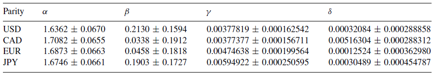
Source: Own elaboration with data from the Bank of Mexico using the STABLE.EXE program.

The stability and asymmetry parameters estimated and presented in Table 2 are consistent with the results obtained by ^{Dostoglou and Rachev (1999)}, ^{Čížek, Härdle, and Weron (2005)}, ^{Scalas and Kim (2006)}, and ^{Climent-Hernández and Venegas-Martínez (2013)}. The stability parameters indicate that the distributions of the yields are leptokurtic, and the asymmetry parameters indicate that the distributions extend toward the right end with greater frequency than toward the left end; concluding that the yields of the exchange rates present leptokurtosis and positive asymmetry.

Kolmogorov-Smirnov goodness of fit test

After the estimation of the α-stable parameters, the quantitative analysis is done to prove the null hypothesis H ₀, which states that the yields of the exchange rate parities present a Gaussian distribution, against the alternative hypothesis H ₁ that states that the yields do not present a Gaussian distribution, using the Kolmogorov-Smirnov goodness of fit statistic presented in Table 3.

Table 3 Results of the Kolmogorov-Smirnov test for the Gaussian distribution. 

Source: Own elaboration in a spreadsheet with the data from the Bank of Mexico.

From the results of Table 3 and with significance levels of 10%, 5% and 1%, it is concluded that the null hypothesis, which states that the yields present Gaussian distributions, must be rejected. Table 4 presents the tests carried out through Lilliefors goodness of fit test for the null hypothesis H ₀, which states that the yields present a Gaussian distribution, against the alternative hypothesis H ₁ that states that the yields do not present a Gaussian distribution.

Table 4 Results of the Lilliefors test for the Gaussian distribution. 

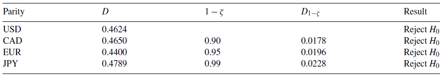
Source: Own elaboration in a spreadsheet with data from the Bank of Mexico.

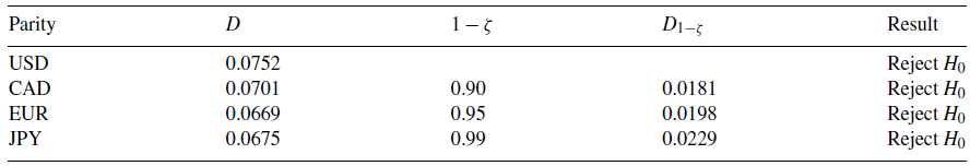
From the results of Table 4 and with significance levels of 10%, 5% and 1%, it is concluded that the null hypothesis, which states that the yields present Gaussian distributions, must be rejected. Table 5 presents the tests carried out through the Kolmogorov-Smirnov goodness of fit statistic for the null hypothesis H ₀, which states that the yields present an α-stable distribution, against the alternative hypothesis H ₁ that states that the yields do not present an α-stable distribution.

Table 5 Results of the Kolmogorov-Smirnov test for α-stable distributions. 

Source: Own elaboration in a spreadsheet with data from the Bank of Mexico.

From the results of Table 5 and with significance levels of 10%, 5% and 1%, the conclusion is to not reject the null hypothesis that states that the yields of the exchange rate parities present α-stable distributions.

Anderson-Darling goodness of fit test

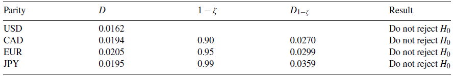
Another test for the null hypothesis H ₀, which states that the yields present a Gaussian distribution, against the alternative hypothesis H ₁ that states that the yields do not present a Gaussian distribution is carried out through the Anderson-Darling goodness of fit test, presented in Table 5.

From the results of Table 6 and with significance levels of 10%, 5% and 1%, it is concluded that the null hypothesis, which states that the yields present Gaussian distributions, must be rejected. Table 7 presents the tests carried out through the Anderson-Darling goodness of fit test for the null hypothesis H ₀, which states that the yields present an α-stable distribution, against the alternative hypothesis H ₁ that states that the yields do not present an α-stable distribution.

Table 6 Results of the Anderson-Darling test for the Gaussian distribution. 

Source: Own elaboration in a spreadsheet with data from the Bank of Mexico.

Table 7 Results of the Anderson-Darling test for α-stable distributions. 

Source: Own elaboration in a spreadsheet with data from the Bank of Mexico.

From the results of Table 7 and with significance levels of 10%, 5% and 1%, the conclusion is to not reject the null hypothesis that states that the yields of the exchange rate parities present α-stable distributions. Therefore, it is concluded that the yields of the USD, CAD, EUR and JPY exchange rate parities present α-stable distributions in fractional probability spaces.

Estimation of the self-similar exponent

The estimation of the self-similar exponent is carried out through the EHG(1) method that presents the expected value E(H)=α ^-1 , which is the limit between anti-persistence and persistence for the α-stable process to obtain the (α, H) pair and to know whether the process is anti-persistent, independent or persistent. The estimations of the exponents through the regressions are presented in Table 8.

Table 8 Estimation and statistics of the self-similar exponents. 

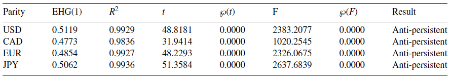
Source: Own elaboration in a spreadsheet with data from the Bank of Mexico.

From the results of Table 8, it is concluded that the parities are anti-persistent in the sense that they do not present the yields expected of α-stable series with αH> 1, presenting the expected positive yields according to the average and the location parameter, which present positive trends but with mean reversion, that is, αH≤1. Table 9 presents the self-similar exponents through the EHG(1) methodology.

Table 9 Estimation, ranges and standard deviation of the self-similar exponents. 

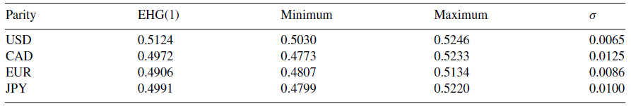
Source: Own elaboration in a spreadsheet with data from the Bank of Mexico.

The results from Table 9 confirm that the parities are anti-persistent, presenting the expected positive yields according to the average, and the location parameter presents a positive trend but with a mean reversion.

The linearity of the EHG(q) regressions, for the q=1,..., 10 moments, determines if the series is self-similar or multifractal. Table 10 presents the estimation of the coefficients of the slopes of the regressions.

Table 10 Estimation and statistics of the coefficients of the slopes of the EHG(q). 

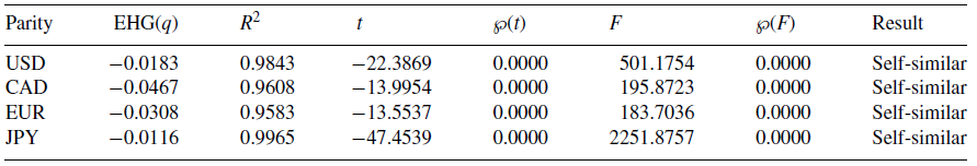
Source: Own elaboration in a spreadsheet with data from the Bank of Mexico.

The results from Table 10 confirm that the parities are self-similar, therefore, the estimations of the α-stable parameters and the KS and AD hypothesis tests indicate that the estimated distributions are more efficient than the Gaussian distribution. This is complemented with the estimations for the self-similar exponents through the EHG(q), the t and F statistics indicate that the series are self-similar and that they are not multifractal. Thus, the assumption of the Gaussian distribution of the yields of all the analyzed exchange rate parities is rejected, while the hypothesis of α-stable distributions of the yields of the USD, CAD, EUR and JPY exchange rate parities is not rejected. Figure 3 presents the (α, H) pairs of the USD, CAD, EUR and JPY exchange rate parities.

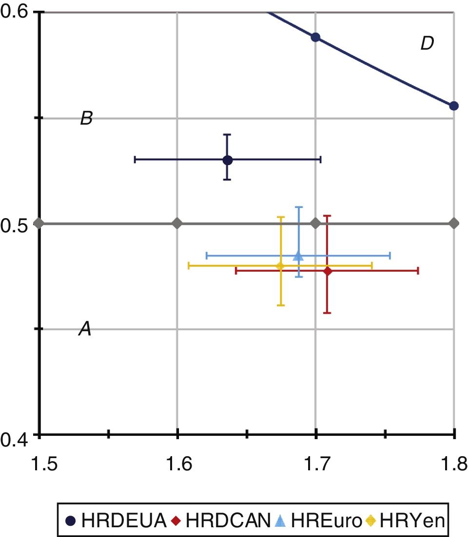
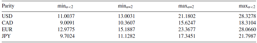
Figure 4 shows that the (α, H) pairs of the exchange rate parities are found in the A and B regions, which represent the MELF which is H-asie and anti-persistent, with the ranges [0.5030, 0.5246], [0.4773, 0.5233], [0.4807, 0.5134] and [0.4799, 0.5220] for the USD, CAD, EUR and JPY exchange rateparities, respectively; where theestimation of the self-similar exponents 0.5124, 0.4972, 0.4906 and 0.4991 are the averages of the regressions for τ = 5,..19 and represent the probabilities of increment for the exchange rate parities, respectively, which present a positive trend during the studied period. Figure 4 presents the accrued yields of the USD, CAD, EUR and JPY exchange rates, respectively; the averages of ten thousand persistent simulations of the fBm with self-similar exponents of 0.80, 0.70, 0.75 and 0.77 for the accrued yields of the USD, CAD, EUR and JPY exchange rates, respectively; and the averages of ten thousand simulations of the ME with the estimated α-stable parameters presented in Table 2, and which correspond to each exchange rate parity.

Source: Own elaboration in a spreadsheet with data from the Bank of Mexico.

Figure 4 Location of the (α, H) pairs of the parities. 

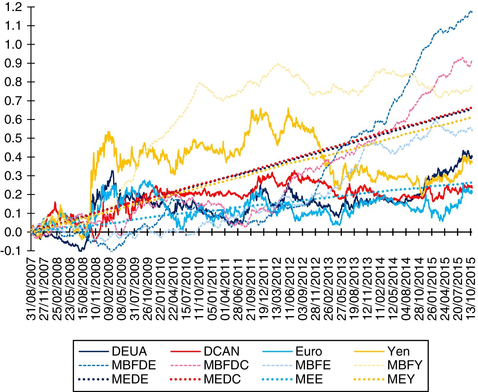
Figure 5 presents the accrued yields of the USD, CAD, EUR and JPY exchange rates, respectively, as well as the averages of ten thousand simulations of the fBm with persistent self-similar exponents and the averages of ten thousand simulations of the ME with the estimated parameters. It can be observed that the accrued yield of the USD is lower than the averages of the simulations of the persistent fBm of the American dollar (USDfBm) and the simulations of the ME of the American dollar (USDME). The accrued yield of the CAD is lower than the averages of the simulations of the persistent fBm of the Canadian dollar (CADfBm) and the simulations of the ME of the Canadian dollar (CADME). The accrued yield of the EUR is lower than the averages of the simulations of the persistent fBm of the EUR and the simulations of the ME of the EUR (EURME). Finally, the accrued yield of the JPY is lower than the averages of the simulations of the persistent fBm of the JPY (JPYfBm) and the simulations of the ME of the JPY (JPYME). Therefore, the parities present mean reversion. It can also be appreciated that the α-stable distributions adequately model the financial low-impact changes through the fBm process and the high-impact changes through the Poisson processes. Furthermore, they also adequately model the asymmetry of the yields that the fBm cannot capture given the fact that it is symmetrical. It can also be observed that the parities present a self-similar exponent that is close to a mean and represents pink noise, in the context of α-stable distributions, which is related to turbulence processes presenting an irregular aspect and not a line as is the case of the average of the simulations of the ME, which represents black noise and which has a softer aspect and is present in processes with long-term cycles.

Source: Own elaboration in a spreadsheet with data from the Bank of Mexico.

Figure 5 Accrued yields and simulation averages. 

In order for the parities to present memory loss (white noise) in the context of the α-stable distributions, the self-similar exponent must approach the H=α^-1 value, and for them to present persistence (black noise) the self-similar exponent must satisfy H>α^-1 . Therefore, the exchange rate parities present anti-persistence (pink noise) because H<α^-1 and they present mean reversion and dynamic balance, but given the bias and location characteristics they also present a positive trend that allows to obtain profit in the medium or long-term. However, these are lower on average than the ones presented by the independent α-stable processes (white noise) and the ones presented by the persistent (black noise) α-stable processes.

Estimation of the confidence intervals

If the variable Y~ S(α, β, γ, δ), then:

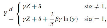
where the random standard variable:

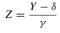
is such that Z~ S(α, β) and the z _ζ th fractal of the random variable is defined as:

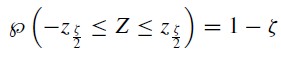
therefore, the confidence interval is:

(3)

where

The confidence intervals of the parities

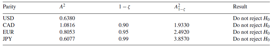
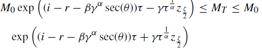
The confidence intervals of the M _T exchange rate parities during period T are estimated through the underlying price M ₀ in the instant t = 0, the national risk-free interest rate i, the foreign risk-free interest rate r, the stability parameter α, the asymmetry parameter β and the scale parameter γ for each of the parities, the corresponding fractals according to the level of significance ζ, and the remaining period τ=T-t for those that require the estimation of the confidence level. The α-stable confidence intervals for the 118 days following the period of study, with a significance level of 1%, are shown in Table 11.

Table 11 Confidence intervals with significance levels of 1%. 

Source: Own elaboration in a spreadsheet with data from the Bank of Mexico.

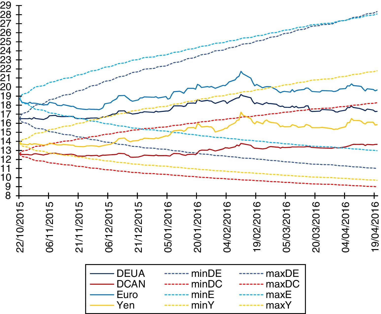
The values in Table 11 show that the α-stable confidence intervals comprise the Gaussian confidence intervals. Said values also model the asymmetry of the exchange rate parities and, in all cases, it is expected for the increments to be superior to the decrements parting from the exchange rate parities as of October 22nd, 2015. The α-stable confidence intervals of the exchange rate parities are presented in Figure 5.

Figure 6 shows that the USD, CAD, EUR and JPY exchange rate parities are within the lower limits (minUSD, minCAD, minEUR, minJPY) and the upper limits (maxUSD, maxCAD, maxEUR and maxJPY) of the α-stable confidence intervals during the period of 10-23-2015 and 04-20-2016. The Gaussian confidence intervals of the exchange rate parities are presented in Figure 6.

Source: Own elaboration in a spreadsheet with data from the Bank of Mexico.

Figure 6 α-stable confidence intervals with significance levels of 1%. 

Figure 7 shows that the USD, CAD, EUR and JPY exchange rate parities are within the lower limits (minUSD, minCAD, minEUR and minJPY) and that the USD, CAD and EUR parities are within the upper limits (maxUSD, maxCAD and maxEUR) of the α-stable confidence intervals during the period of 10-23-2015 and 04-20-2016. The exchange rate parity of the JPY surpasses the upper limit (maxJPY) on February 11th and 12th, 2016. As can be observed, the Gaussian confidence intervals are symmetrical.

Source: Own elaboration in a spreadsheet with data from the Bank of Mexico.

Figure 7 Gaussian confidence intervals with significance levels of 1%. 

The α-stable distributions adequately model leptokurtosis, asymmetry, fluctuations far from the mode or extreme values, and the stability or persistence property of the yields, as they are an effective alternative to model financial and economic series with high-volatility clusters, extreme values with frequencies that are higher than those expected by the Gaussian distribution and that have a financial and economic impact that turns into profit or losses. Furthermore, they satisfy the generalized central limit theorem because the yields are found in the domain of attraction of an α-stable law where the Gaussian distribution is the limit case when α=2. It has also been demonstrated that it is not efficient to model leptokurtosis, asymmetry, the events far from the location parameter and the stability property observed in the yields of the financial and economic series. On the other hand, the yields that are modeled through the α-stable distributions satisfy the stability property that optimizes the performance of the system, because the α-stable applications are broader than the applications of the Gaussian distribution that considers extreme events of high financial and economic impact as improbable and which are, in reality, more frequent and are more properly considered by the α-stable distributions. This allows to improve the applications in financial engineering, risk administration and appraisal of derived products by more adequately quantifying the risks in the evaluation of forward contracts, futures, swaps, options, structured products, value at risk, investment portfolios, and credit risk. Therefore, it is possible to innovate in the appraisal of insurance for contingencies on natural events, which could be modeled through α-stable distributions and the (α, H) pair that allows to more adequately infer the characteristics of the time series, while structuring more adequate innovative products through financial engineering.

The importance of relating the (α, H) pair allows to infer the risk of the events, because if the stability parameter approaches the unit then there is a high chance of events that will be distant to the ones expected by the Gaussian distribution, which turns into significant profit or losses. It can also be inferred through the asymmetry parameter: if positive, it indicates that the probabilities of profits superior to the average are higher than the probabilities of losses and vice versa. When the stability parameter approaches two, then there is an equivalent probability of events close to the ones expected by the Gaussian distribution. The self-similar exponent allows to infer the behavior that the series presents in the context of the variation that translates into risk due to changes; when the product of the self-similar exponent and the stability parameter is lower than the unit, the series is anti-persistent, presents mean reversion and high variation, which in turn translates into a high risk in the short and medium term. If the product of the self-similar exponent and the stability parameter are close to the unit, the series has memory loss and the positive and negative changes present approximately the same probability of occurrence, which translates into a moderate risk in the short and medium term. When the product of the self-similar exponent and the stability parameter is greater than the unit, the series is persistent, and presents long-term memory and moderate variation, which translates into a low risk in the short and medium term because the changes they present are less pronounced than when the product of the self-similar exponent and the stability parameter is lower than or equal to the unit. Thus, based on the proposal presented in ^{Rodríguez Aguilar (2014)} it is suggested to use the ℵ= αH index to infer the behavior of the series. The estimation and validation of the parameters of the α-stable distributions and the self-similar exponent are important in the creation of innovative investment instruments, using financial engineering and the administration of financial risks. This has been proposed in the works by ^{Climent-Hernández and Venegas-Martínez (2013)}, who estimate the distribution parameters of the yields and carry out qualitative and quantitative analyses to select the best estimation of the α-stable parameters, presenting evidence of the presence of leptokurtosis and asymmetry in the yields and consider the α-stable distributions as a more realistic alternative to model the dynamics of the yields in the evaluation of options. ^{Climent-Hernández and Cruz-Matú (2016)} indicate that in incomplete markets, it is impossible to fully transfer the risks. The lack of completeness of the financial markets presents itself due to the commercialization related to the risks that need to be covered, the lack of knowledge on the appropriate model to model the yields and the discontinuities in prices. The stability parameter provides information regarding the behavior of the process: when it approaches two, the process presents a greater number of oscillations of low financial impact (yields close to zero) among the jumps of high financial impact (yields that generate moderate losses or profit); when it approaches to the unit (Cauchy process), the prices of financial insurance change due to the jumps that generate significant losses or profit and due to the presence of stability periods between the jumps, which are more adequately captured by the log-stable processes since they capture the oscillations of low financial impact through the Wiener process and the high impact jumps that generate significant losses or profit through the Poisson processes. The estimation of the distribution of the yields and the qualitative and quantitative validation allow to observe that the log-Gaussian process overestimates the events that generate losses or profit that are not significant, and underestimates the events that generate losses or profit that are significant. ^{Climent-Hernández, Venegas-Martínez and Ortiz Arango (2015)} indicate that the mean-variance analysis, proposed by ^{Markowitz (1952)}, is one of the first theories that were developed for the problem of optimal portfolio selection, and one of the assumptions is that the yields come from a multivariate Gaussian distribution; however, they indicate that there are conjectures that dismiss the Gaussian distribution. ^{Climent-Hernández (2016)} presents the problem of the optimization of a portfolio when the yields are modeled through log-stable processes, considering the duration and convexity in the debt markets and the non-linearity in the options markets.

The efficient use of the resources needs basic and applied research proposals utilizing information and communications technologies to be in global competition, innovating to satisfy the needs. A change of paradigm is necessary for the simplified theories with a priori hypotheses that are unsatisfactory, where the information is inefficient and competitivity is far from balance due to the nature or social behavior, additionally, the central limit theorem is unsatisfactory. The risk measure that quantifies the deviation of the historical average through the dispersion measure is fundamental in understanding the future behavior of study events, while diversification is important to minimize the risk measure of the system. The conditions change instantly due to significant changes and to stability periods between the significant changes, and are more adequately modeled through log-stable processes since they capture the changes in the periods of stability through the Wiener process and the significant changes in the conditions of the system through the Poisson processes, adequately modeling heteroscedasticity caused by variables with asymmetrical distributions and the presence of extreme values. The theory of extreme values allows extrapolating information from a sample, and the shape of the end of the distribution is estimated. With the sample, it is complicated to find expressions for the distribution of the maximum and thus an approximation to a limit distribution that converges into a degenerated distribution is sought. Under certain circumstances, this pertains to one of the Gumbel, Fréchet or Weibull distribution classes of extreme values, which combine into a distribution with common parameterization or generalized extreme values distribution. The distributions such as t-student, mixed Gaussian and α-stable (generalized Pareto) are found in the domain of attraction of the Fréchet distribution, which is adequate to model financial assets. The distributions such as Gaussian, log-Gaussian, exponential and gamma pertain to the domain of attraction of the Gumbel distribution and the uniform and Rayleigh distributions pertain to the domain of attraction of the Weibull distribution. Generally, they are applied to natural events such as in the distribution of galaxies, the level of seas, rivers or damns, wind speed, pollution concentration, the volume of rain or snow, material resistance, maintenance times or engineering replacements and in the models for insurance, financial engineering and the administration of financial risks. The log-stable processes explain the behavior of the changes, identifying the model through the estimation of the stability, asymmetry, scale and location parameters; verifying assumptions and using the model to describe and infer through the available information. The change in paradigm happens because the language of the nature with Euclidean geometry characters such as triangles, circles, quadrilaterals or regular and irregular polygons is unsatisfactory, that is, the clouds are not spherical or elliptical, the mountains are not conical, the lines of the coasts are not circumferences, the crust of the earth is not smooth, and the light does not travel in a straight line. Therefore, the objects in the real world are not solid because they present irregularities such as spaces and deformations, thus, in a three-dimensional space, the dimension of the objects is fractal and it reflects the properties of the scale and its value is between one and two. The stability, asymmetry and scale parameters of the log-stable distributions, along with the self-similar exponent, allow to know the fractal dimension of the probability space of the changes of the objects in the system. The bias indicates the probability of positive or negative changes in the objects. The scale is the measure of risk or potential change of the objects, and the self-similar exponent indicates the probability that the changes remain according to the trend or for them to revert to the historical average that the objects have presented in the system. This is applicable in natural and social events that are modeled through fractional nature such as factors that attract dynamic systems, surfaces that separate two means, branch systems, porosity, dispersion, migration, colonization, extinction or persistence of species, seismology, nets, video and finances. The ℵ index relates the dimension of the probability space and the self-similar exponent to infer the behavior of the events studied and whether they present mean reversion, independence or long-term memory. If ℵ<1, the events present mean reversion and it is expected for the contrary of what is currently happening to occur eventually, if ℵ≅1, the events are random and if ℵ>1, the events present long-term memory and the expectation is for this to continue happening with a higher probability of the contrary happening eventually. The scale and stability parameters of the log-stable distributions and the self-similar exponent are important in their own right, because the dimension of the probability space or the dimension of the time series, along with the risk measure, indicate which events are riskier. The USD and CAD exchange rate parities present log-stable distributions in probability spaces with dimensions of 1.6362 and 1.7072, respectively, and the series have dimensions of 1.4876 and 1.5028, respectively, through the self-similar exponent, and have dimensions of 1.3888 and 1.4146, respectively, through the stability parameter. This means that the dimension of the USD is smaller than that of the CAD and if both present risk measures hypothetically equal to 0.0038, the investors have tools to know with more certainty that the events of the CAD are riskier than those of the USD because the yields take a bigger surface on the plane, therefore, indices Ω=αγ and Ʊ=Dγ can be calculated to know the events that present a greater risk.

Conclusions

The estimations of the α-stable parameters and the KS and AD hypothesis tests indicate that the estimated α-stable distributions are more efficient than the Gaussian distribution to quantify market risks. The estimations of the self-similar exponents and the t and F statistics indicate that the series are self-similar and that they are not multifractal, rejecting the Gaussian distribution of the yields of all the analyzed parities and not rejecting the α-stable distributions of the analyzed yields.

The importance of the (α, H) pair allows to infer the risk of the events, given that if ℵ<1 the series is anti-persistent, has a short-term memory, mean reversion, negative correlation and elevated variation, with a high risk at the short and medium term because D>2-α^-1. When ℵ=1, the series is independent, has memory loss, null correlation, and the positive and negative changes present approximately the same probability of occurrence, with a moderate risk at the short and medium term because D=2-H=2-α^-1. If ℵ>1, the series is persistent, presents long-term memory, a positive correlation and moderate variation, with a low risk at the short and medium term because D<2-α^-1 and the changes that present themselves are smaller than when ℵ≤1 and D≥2-α^-1. The γ scale parameter presents a direct relation with the risk; when y approaches zero, the risk decreases because the series presents events that are close to the ones expected when these high frequency events and their financial and economic impact do not generate large profits. If γ increases, the risk increases because the series presents events that are distant from the ones expected with high frequencies and large profits or losses. The β asymmetry parameter is related to the frequencies of the movements of the series. If β<0, the series presents events with negative movements with a higher frequency and more distant to the expected events than the positive events, which generates large profits or losses depending on the posture that the investors acquire with respect to the subjacent, which are heightened by the βγ ^α scale parameter. The difference between the i-r risk-free interest rates is added to the asymmetry parameter to indicate the trend of the series. Therefore, the estimation and validation of the parameters of the α-stable distributions and the self-similar exponent are important in the creation of innovative investment instruments, utilizing financial engineering, risk administration and the appraisal of derived products, as has been proposed in the works by ^{Climent-Hernández and Venegas-Martínez (2013)}, ^{Climent-Hernández et al. (2015)}, ^{Climent-Hernández (2016)}, and ^{Climent-Hernández and Cruz-Matú (2016)}.

The fractal dimension of the probability space, the dimension of the time series, the self-similar exponent, and the scale parameter are individual indicators that show the characteristics of the bias and dispersion of the events. Generally, the ℵ index indicates the correlation that the events present through time and their estimation is important to infer the behavior of natural and social events.

It is possible to evaluate, in future finance research works, products that are structured around forward contracts, futures, swaps or options with different characteristics, while innovating with other types of coverages. In other branches of science, it is possible to evaluate natural or social events that are modeled through log-stable distributions and that are related to the self-similar exponent.