The slow growth, manufacture and employment in Mexico

In the last three decades, the Mexican economy has experienced a lower growth rate than what it had at the beginnings of the 1980s. This performance has been explained through different arguments, but there is a central point worth mentioning that refers to the effects that the growth of economic activity has had in the generation of employment.

With regard to this point, some authors (^{Calderón & Sánchez, 2012}) have analyzed the low economic growth in Mexico and the impossibility to generate the necessary jobs. They specifically provide evidence of the high correlation between the low economic growth of the total GDP and the low growth of the manufacturing output. According to these authors, between 1982 and 2010, the Mexican economy grew 2.1% per year. Associated to this phenomenon is the high unemployment and the employment instability: between 1892 and 2008 only an average of 354,306 jobs were created per year in the formal sector of the economy.

In this sense, an important part of the explanation of the deficiency of the formal economy to generate the jobs demanded by the labor market is in the importance of the dynamic of the economic activity of the country. If the growth rate of the real GDP and total employment for the Mexican economy are reviewed within a relatively long period, the observed tendency is that the crisis of 1982 marked the end of a relatively high output growth phase with relatively high rates (6.8 yearly average between 1970 and 1981) and the start of a slow growth process. In the period of 1982-2013 the average growth of the real GDP was of 2.3%, whereas the growth of employment was of only 1.2% (see Fig. 1).

Fig. 1 Mexico: Real gross domestic product and total employment, 1971-2014. Growth rates. 

This is important because it suggests reviewing what is happening with the sectoral production in order to identify if this slow growth process has spread in similar magnitudes to the sectors of economic activity.

Table 1 shows the changes to the structure of the GDP and total and sectoral employment in detail. First, it is evident that for the entire period of 1970 to 2014 the average growth of 3.5% of the real GDP has not been enough for the total employment to grow in a significant manner (having grown an average of 1.9% per year for this period). It stands out that the services sector is the one that has grown the most, with a yearly average growth rate of 3.8% for the real GDP and 2.7% for employment, whereas in manufacturing, even with an average growth rate 3.5% for the real GDP, employment has only grown by an average rate of 0.9%, just above the agriculture and livestock sector. Furthermore, it must be noted that according to the standard deviation of the manufacturing GDP, it is a sector with significant fluctuations regarding the median, contrary to what occurs with the service sector. Moreover, the manufacturing sector is very sensitive to the fluctuations of the Mexican economy and the external sector, and as such has reported years with heavy drops and boom periods with significant growth rates.

Table 1 Mexico: Growth rate of the real GDP and employment, total and sectoral. Basic statistics by periods, 1970-2011. 

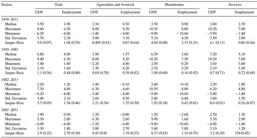
Source: Elaborated with data from the System of National Accounts (INEGI, 2012, 2014a,b).

If we divide the period of 1970-2011 into two sub-periods (1970-1981 and 1982-2011) to identify the changes in the structure of the sectoral employment following the crisis of 1982, which has become the starting and breaking point of a growth model based on external demand and has given way to the low growth phase of Mexico, we find some significant regularities in an aggregated manner.

It is clear that between 1970 and 1981, the final phase of the Mexican miracle was experienced with relatively high growth rates for the Mexican economy, with a 6.8% yearly average for the total GDP and a 4.0% yearly average for the total employment, and a dynamic manufacturing sector with an average GDP growth of 6.3% per year (with some years having growth rates for the real GDP of 10.2%) and an average employment growth of 3.6% per year. This period, which was relatively dynamic for the three production sectors, significantly changed at the start of the 1980s (see Table 1).

For the period of 1982-2011 manufacturing stopped growing at the rates that characterized it until before the crisis of 1982 and has followed a similar tendency to the behavior of the Mexican economy with an average rate of 2.4%, but with a negative employment growth rate of −0.1%

The scenario becomes complicated if we analyze the period of 2001-2011, during which the average growth of manufacturing was not only lower (1.2%), but on average, employment presented negative growth rates of −2.6%, these being lower than even those of the agriculture and livestock sector which is a net ejector of employment (see Table 1). The explanation for this decrease in the growth of the manufacturing activity is that since 2000, Mexico's foreign commerce has not experienced the dynamism of the period from 1993 to 2000, particularly due to the competition with China and the continued disintegration of the NAFTA (^{Dussel Peters & Ortiz, 2012}).

In this sense, ^{Dussel Peters (2003)} notes that the capacity for the generation of employment of the manufacturing sector has been drastically reduced, as the average growth of employment during these years has been negative, which indicates that the sector has ejected work. This evidences the decrease in its capacity to drive the economic activity of the country. On the other hand, the author also argues that perhaps the results could be explained by the fact that starting on 1988, manufacturing specialized in capital intensive exporting activities, which has generated a reduced process for employment creation.

On the other hand, ^{Dussel Peters and Ortiz (2013)} highlight a systematic drop of the relative weight of the permanent manufacturing employment with regard to the total permanent employment, from 35.6% in 2000 to 26.1% in October 2012. Moreover, they note that employment in the manufacturing sector was one of the most affected by the economic crisis of 2008, given that of the 701 thousand permanent jobs lost between October 2008 and May 2009, 349 thousand corresponded to the manufacturing sector. This means that 1 of every 2 permanent jobs during these months corresponded to manufacturing activities, which translates to a drop of 9.2% on the expansion rates of the permanent manufacturing employment.

With this significant decrease in the generation of employment of the manufacturing sector, another fundamental change is the continuous expansion of the service sector, both due to its relative weight in the economy as well as its strategic role in the functioning of the productive systems (^{Chávez & Zepeda, 1996}). Thus, the employment structure by sector of activity has changed in a significant manner in recent decades. The service sector gains increasing importance in contrast to the industrial and agriculture and livestock sectors. Fig. 2 shows the significant increase in employment in the service sector, whereas since the crisis of 1982 manufacture has stopped growing at its previous levels, in fact, a persistent drop in the employment levels of this sector starting in 2000 is clear, and becomes more pronounced since 2008.

Fig. 2 Mexico: Percentage structure of the sectoral employment, 1970-2012. 

This reorganization of the sectoral employment structure is relevant from different perspectives. First, because “manufacture is important to absorb workers with little training, being the sector from which the middle class emerges and grows worldwide” (^{ONUDI, 2013}); it is considered an activity with unique characteristics: its forward and backward connections, its potential in the generation of value added, of technology diffusion, of growth of productivity and, of course, as a generator of formal employment (^{Dussel Peters, 1997}). Furthermore, it generally provides greater benefits and safety to the workers than jobs in other sectors, and tends to develop better abilities than equivalent jobs in the rest of the economy (Lavopa and Szirmai, 2012, cited in ^{ONUDI, 2013}).

Thanks to the dynamism of manufacture, its effects transfer to other sectors of activity, inducing innovating behaviors on the economic agents (^{Garduño, 2009}). The service sector represents the opposite case, especially because it incorporates an important part of informal employment.

Regarding this point, ^{Dussel Peters and Ortiz (2013)} note that since the year 2000 employment has redirected the service industry, and manufacturing has lost 9.5 percentage points in the generation of employment between 2000 and November 2013, whereas the services to companies and people have increased their percentage participation by a little more than 5.0%. In this reorganization, agricultural employment continues the tendency that has characterized it in recent decades: a sector with a decreasing dynamic in the generation of employment and an ejector of workforce.

In the case of the regions of Mexico, ^{Sánchez (2011)} analyzes the economic stagnation that prevails in Mexico since 1982 and demonstrates, in the framework of the Kaldorian analysis, that the insufficient dynamic of the manufacturing sector is the main cause of the low economic growth and employment rates in the regions of Mexico and in the country in general. Specifically, the existence of a vicious cycle between the low growth in production and the low growth in employment stands out (which leads to low incomes and thus a limited market growth), which perpetuates the vicious cycle of economic stagnation.

The regions of Mexico are clearly no strangers to this tendency, especially because the productive activity has not responded to the pressure exercised by the economically active population on the job market, and because manufacture, as the most dynamic sector, is certainly causing a decrease in the number of jobs. In this context, the case of the Central region of Mexico is specifically addressed in the following section.

The structure of employment and the production of manufacture by major division in the Central region of Mexico

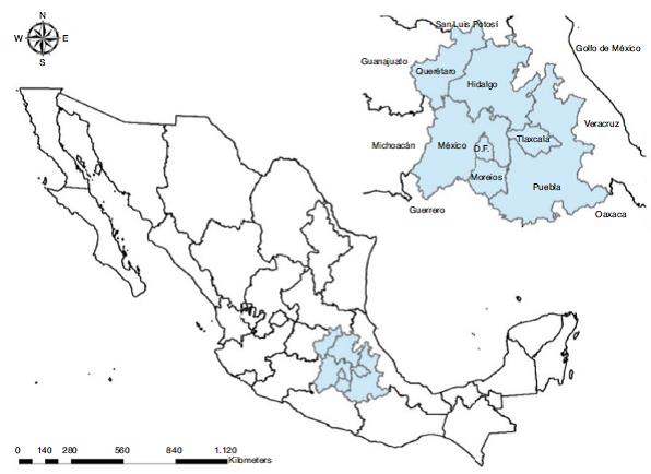
As noted, it is the case of the Central region of Mexico that is being addressed, comprised by Mexico City, the State of Mexico, Querétaro, Puebla, Hidalgo, Morelos and Tlaxcala (see Fig. 3). These states, in addition to their geographical location, have the presence of the manufacturing industry as one of the main economic and employment generation activities in common.

Fig. 3 Central Region of Mexico. 

Mexico City and the State of Mexico symbolize the cradle of the industrialization process in Mexico, and even though in recent years a “deindustrialization” process has been made manifest, in the sense that the growth rates of industrial activities have decreased in comparison with previous years, they prevail as the two most representative entities at the national level. In 2012, their contribution was of 26.2% to the total national GDP, and 20.4% to manufacturing (^{INEGI, 2014c}), in addition to being the most populated states in the country and together comprise 24 million people (21.4% of the national total) (^{INEGI, 2010}).

In the other states, manufacturing activities though in recent years they have lost representativeness regarding the activities of the secondary sector have a significant participation within the state productive structure. The contributions to the total GDP of each state are the following: Querétaro 28.7%, Puebla 24.4%, Hidalgo 33.4%, Morelos 24.3% and Tlaxcala 29.7% (^{INEGI, 2014c}).

Although the weight of the manufacturing industry has decreased with regard to the service sector, there can be no doubt that it continues to be a sector whose activity is highly important in driving the aggregated economic activity of the regions and the country and, consequently, employment. Some authors that have analyzed the “backwards” productive connections of manufacture, provide evidence of its driving capacity and report a direct and total driving capacity of 1.63 times, above the tertiary sector (1.36 times) and the primary activities (1.31 times). That is, the evolution of the Mexican economy significantly depends on the performance of its manufacturing industry (see^{Guerrero de Lizardi, 2012}).

In this sense, it is important to analyze the performance shown by the manufacturing industry in order to identify the most dynamic divisions of activity in each of the states of the Central region.¹

According to the indicator of the evolution of the manufacturing production per major division, its performance in recent years has not been homogeneous. Divisions II and III have stagnated, particularly after the year 2000, whereas divisions VIII and IX have stood out because after the 1995 crisis their evolution has been above the rest of the manufacturing divisions (see Fig. 4).

Fig. 4 Mexico: Evolution of the GDP of manufacture per major division, 1988-2012. Index 1988=100, at constant 2003 prices. 

Although the dynamism of the different manufacturing divisions is not the same, in most of them a process of growth can be observed; however, this tendency contrasts with what can be observed regarding employment. In particular, after the year 2000 the employment levels have decreased for all the divisions, which denotes a growth process without consequential effects in the volumes of employment. Even the decreasing tendency of recent years would entail a loss of formal employments (see Fig. 5).

Fig. 5 Mexico: Evolution of the employment of manufacture per major division, 1994-2012. Index 1994=100. 

For the case of the Central region, this tendency has not changed in a significant manner. Specifically, some authors report that the region has lost representativeness in the ensemble of economic activity, whereas other regions (especially those in the north) have gained participation. ^{Sánchez (2011)} states that between 1993 and 2010 the average annual growth rate of manufacture was of 2.68% for the entire country. In the North-central region, the growth rate was of 5.54%, 4.11% in the Northern Border, 1.71% in the Pacific, 1.70% in the Southern region, 1.54% in the Gulf, 1.43% in the Western region, and only 1.35% in the Central region. This last region, as stated by ^{Sánchez (2011, p. 104)} “after having been the industrial center of the country it has gradually ceased to be so”. In recent years, there has been a clear shift of the manufacturing activities in favor of the northern regions of the country.” Moreover, “… it is in clear decline, in only four years it managed to show a growth above 5% and in 2009 it was the region most affected by the crisis by decreasing its yearly production by 8.5%” (^{Sánchez, 2011}, p. 107).

^{Calderón and Martínez (2005)} conclude that the analysis of the distribution of employment by regions reveals that starting with the process of trade openness, the Northern region has had a growing participation, whereas the Central region shows a rather significant drop in manufacturing employment, remunerations, and the value added of this industry.

Although the evidence presented for manufacture shows heterogeneities in the growth by regions, it is also important to analyze what happens by division of activity, especially because the nine major divisions that comprise the manufacture sector are not homogenous in their structure and respond differently to the fluctuations of the global economy.

From the census information of 1985, 1988, 1993, 1998, 2003 and 2008 (INEGI, various years) some regularities at the manufacture activity division level can be observed for two periods: 1985-1993 and 1993-2008.

Generally speaking, the Central region is one in which the growth of the economic activity, measured through the census real gross value added (valor agregado censal bruto real, VACBR), is low and even negative in some activity divisions, and the changes that manifest between the two periods are not significant due to their scale. However, some states stand out due to the dynamic, or significant drops, that some activity divisions present (see Table 2), as described below.

Table 2 Central Region: real gross value added and employment. Average annual growth by periods, 1985-2008. At constant 2004 prices. 

Source: Elaborated with data from the Economic census 1985, 1988, 1993, 1998, 2003 and 2008 (INEGI, 1986, 1989, 1994, 1999, 2004, 2009).

Note: Division I: Food products, beverages and tobacco; Division II. Textiles, clothing and leather industry; Division III. Timber industry and wood products; Division IV. Paper, paper products, print and publishers; Division V. Chemical substances, petroleum derivatives, rubber products and plastics; Division VI. Non-metallic mineral products, except petroleum and carbon derivatives; Division VII. Basic metallic industries; Division VIII. Metallic products, machinery and equipment; Division IX. Other manufacturing industries.

In the case of Division I. Food products, beverages and tobacco, the region as a whole presents a decrease in the average annual growth of the VACBR (from 2.16% between the period of 1985-1993 to 1.77% for the period of 1993-2008), though the states of Hidalgo, Puebla, Querétaro and Tlaxcala stand out due to their growth; specially Hidalgo, which for the two periods has had average annual growths at rates of 8.0% and 7.5%, respectively. The particularity of Puebla, Querétaro and Tlaxcala is that from one period to the next they grew significantly, even up to seven times more in the case of Tlaxcala. The State of Mexico has practically maintained its growth levels (see Table 2).

For Division II. Textiles, clothing and leather industry the period of 1993-2008 became a recovery phase, in the sense that in the total of the region between 1985 and 1993, this division presented negative average growth rates. However, the case of Hidalgo stands out, which went from registering drops in production of close to 9.0% between 1985 and 1993 to having annual growth rates of 2.12% for the period of 1993-2008; as does the case of Tlaxcala, that for the same periods had average growth rates of −6.07% and 3.51%, respectively. It is worth mentioning the consolidation process of Querétaro, which has gradually presented consistent growth in this division of activity (see Table 2).

Division III. Timber industry and wood products is relatively strong for some states of the region, specifically Morelos, Puebla and Tlaxcala. Between the two analysis periods a significant growth is registered in the economic activity of this division (see Table 2), which contrasts with the relative stagnation of the evolution of this division for the total of the Mexican economy (see Fig. 4).

In the case of Division IV. Paper, paper products, print and publishers a deceleration process for Mexico City regarding the growth of this activity, and a significant growth for Hidalgo, Querétaro and Tlaxcala (7.2%, 8.7% and 14.25%, respectively, for the period of 1993-2008) is observed. In addition to the difficulties of the State of Mexico and Morelos to reactivate growth in this activity. In the case of Puebla, a recovery is registered for the years after 1993 (see Table 2).

Division V. Chemical substances, petroleum derivatives, rubber products and plastics is a division in which significant recovery processes have taken place in the states of Mexico, Morelos, Puebla and Querétaro, however, the decrease in growth in the rest of the states that comprise the Central region has also intensified, particularly in the state of Hidalgo (see Table 2).

For Division VI. Non-metallic mineral products, except petroleum and carbon derivatives relatively high growth rates are observed for most of the states in the region for the period of 1993-2008. The case of Tlaxcala stands out, with a production growth that reaches average rates of 12.7%. Mexico City and the State of Mexico also stand out, registering negative rates of 11.8% and 0.34%, respectively (see Table 2).

According to the information, it seems that Division VII. Basic metallic industries hasbeen among the ones that have lost in this globalization processes, at least in the Central region. The average growth rates registered for the states are negative for both periods, except for Querétaro which reports a significant growth between 1993 and 2008 (see Table 2).

The case of Division VIII. Metallic products, machinery and equipment has a high note, especially because it is one of the divisions of activity with greater possibilities of generating production expansion dynamics and greater value added because, among others, it includes the automotive sector, which has become a reference in the process of innovation and production growth. In this division of activity, the states of Mexico, Puebla, Querétaro and Tlaxcala stand out, having strengthened their production growth between 1993 and 2008. This is important because it implies greater value added activities, which have greater possibilities of influencing the generation of employment. The case of Tlaxcala, which in the period of 1993-2008 had an average annual growth of 8.2%, and the cases of Mexico City and Hidalgo, which register significant drops in their economic activity (see Table 2) stand out.

Finally, Division IX. Other manufacturing industries registers significant growths in both periods. Puebla in particular has become the state in which this division of activity has consolidated due to its economic activity levels (21.7% for 1993-2008), which means significant effects in the creation of employment.

According to these data, the central region is generally in a process of manufacturing production growth similar to what is reported by ^{Sánchez(2011)} in the sense that the region has gradually stopped being the industrial center of the country. Although, there are divisions of activity that have driven the growth of manufacture in some of the states, among them Puebla, Querétaro and Tlaxcala. In these conditions, the effects at the job creation levels are evident, especially because according to the Keynesian arguments there is an important correlation between economic activity and employment, which is explained by the weight of the effective demand.

In this manner, the data from Table 2 evidence this relation and the following regularities are identified: (a) even when in some divisions of activity a deceleration is reported in the growth of the VACBR, the degrees of the average growth of employment are greater, especially in divisions I, II, III, V and VI; (b) the divisions that comprise the more technical branches, with greater innovation processes and which are strongly based on exports, such as division III, present a lower ratio between economic activity growth and employment growth; (c) these relations allow assuming that the employment income elasticity of the sectors linked to the external sector, such as division VIII, is less than those that respond more to domestic demand factors.

The statistical information approach approximates us to the analysis of what is happening with the growth of the economic activity and employment in the divisions of manufacturing activity in the Central region of Mexico. This is important because it assumes that this production growth tendency, analyzed from the Central region, could contribute to the explanation for Mexico's slow growth and the problem in the creation of employment; especially in the manufacturing sector which, as has already been mentioned, is a sector that has decelerated significantly, affecting the creation of formal employment.

Based on this diagnosis, a function of employment is estimated in the following section, using panel data for each of the divisions of manufacturing activity in order to identify elements that explain the evolution of employment in the Central region.

The theoretical arguments of labor demand

Normally, studies on employment depart from the explanation of the behavior of the job market using employment offer and demand functions. In these cases, the theoretical argument focuses mainly on elements of a neoclassical or Keynesian character. For the purposes of this work Keynesian arguments are used, specifically from the New Keynesian Economics school (NKE) which assumes that the employment level depends on the effective demand and that unemployment can be explained through the existence efficiency wages higher than the equilibrium wages. The fact that employment depends on the effective demand is explained by Keynes’ proposals in the sense that when a company satisfies the demand for their product, it employs the exact quantity of work necessary to meet the demand. If more work is needed to produce a greater quantity, the companies must employ more work when the production demand is higher (^{Abel & Bernanke, 2004}), thus it is considered a positive relation between production and employment.

Here, the NKE has tried to explain performance based on the existence of a real wage that equilibrates the job market and which is essentially rigid. While the neoclassical model postulates the dependency of the wage of the level of productivity, some authors of the NKE invert the terms of the relation and present the possibility that it is productivity that positively depends on the wage. Their main hypothesis is that, though the payment of a higher wage generates greater costs for the company, it also provides more benefits due to its positive impact on the effort of the workers and, ultimately, on productivity. Efficiency wages would be the quantities that the companies would pay above the market value of the equilibrated wage to avoid drops in productivity (^{Gordon, 1990}; ^{Malcomson, 1981}).

According to ^{Mankiw and Romer (1991)}, the existence of this type of wages could be attributed to three reasons: (a) that a higher wage can contribute to increase the effort of the employees and, therefore, positively affect their productivity; (b) an elevated wage can also contribute to improve the capabilities of the employees. Thus, if it is assumed that the wages of the qualified employees are greater and that the company decides to pay wages above the equilibrated market value, more skilled workers will be drawn to the company and, therefore, the average productivity of its employees will increase; (c) a higher wage can stimulate a feeling of loyalty in the employees and prompt a greater effort.

In this discussion, it is considered important to retake the arguments of the New Keynesian Economy to try and simplify the analysis of employment by highlighting the relation between product (via effective demand) and employment, as well as that of real wage (under the hypothesis of the efficiency wage) and employment. The analysis is complemented with the inclusion of an economy diversification index that represents an empirical measurement of the agglomeration economies to analyze the local economic structure. In this case, the diversification variable makes it possible to measure the type of industrial structure by evaluating if it is diversified or concentrated (see ^{Sobrino, 2003}) and, consequently, the effects that it could have in the creation of employment. A positive correlation is expected between economic diversification and employment to greater diversification, greater employment especially due to the heterogeneity in the qualification of the workforce of the regions.

Empirical evidence

Panel specification

Nine panels were integrated, one for each major division of activity of the manufacturing industry as indicated in the note in Table2. They are balanced panels withn= 7,T= 6 andN= 42, that is, they consider the 7 states that comprise the Central region of Mexico, with cross sections of six periods that correspond to the information of the Economic census of the ^{INEGI for 1986}, ¹⁹⁸⁹, ¹⁹⁹⁴, ¹⁹⁹⁹, ²⁰⁰⁴ and ²⁰⁰⁹, with 42 observations.

We worked with the following variables for each of the nine divisions of activity of the manufacturing industry: employed personnel, total remunerations for the employed personnel, census gross value added, and labor productivity, and an economic diversification index was created as indicated below. In the Census of 1986, 1989 and 1994 the INEGI reported the statistical information of the manufacturing sector at the nine major divisions level. However, in the Census of 1999, 2004 and 2009, the information of the manufacturing sector is disaggregated into twenty-one sub-sectors. It was, therefore, necessary to group the sub-sectors in order to homogenize the information at the nine major division level, the way it was previously recorded.

The general specification of a linear regression model with panel data is the following (^{Hsiao, 2003}):

(1)

where i refers to the individual or to the unit of study (cross section), t refers to the dimension in time, α is a scalar, β is a vector of K parameters, X_it is the i th observation at time tf or the K explicative variables, and uit is the error term.

In this case, the total sample of the observations in the model would be given by N×T, where N is the number of individual units of study and T is the period of time.

The panel models can be interpreted through their error components. The error term uit included in (1) could be broken down as follows:

where δit denotes a non-observable variable that remains constant throughout time for each observation (non-observable individual effect), δt represents the non-quantifiable effects that vary with time but not between the units of study, and eit refers to the error term. Most of the applications with panel data utilize the error component model in one direction: u_it=μ_i+e_it, for which δt=0 (see ^{Baltagi, 2005}: chapter 3).

Based on the different assumptions regarding the specific effects μ_i, three possibilities could be present: (a) when considering that μ_i= 0, that is, that any non-observable heterogeneity exist between the individuals (thus grouped regression is employed); (b) when it is assumed that μ_i is a fixed effect and different for every individual, so that the linear model is the same for all the individuals, but the ordinate origin is specific for each of them. Consequently, in this case, the non-observable heterogeneity is incorporated to the constant of the model; and (c) when μ_i is treated as a non-observable random variable that varies between individuals but not in time. In this case, the non-observable differences are incorporated to the error term.

These variants regarding the non-observable heterogeneity give rise to two types of models: the fixed effects model and the random effects model (^{Montero, 2007}; ^{Wooldridge, 2002}).

The fixed effects model

(2)

It assumes that the u_it error expressed in (1) can be broken down into a purely random eit part and a fixed constant, different for each μ_i individual (considered a parameter to be estimated for each observation), which is equivalent to carrying out a general regression and provide every individual with a different point of origin (ordinates), thus incorporating heterogeneity to the constant model α_i=α+μ_i. In this way, in the fixed effects model the uit are treated as a set of additional n coefficients that can be jointly estimated with the β_s. Moreover, the fixed effects model assumes that the individual effect is correlated with the other regressors, that is, cov(X_it,μ_i)≠0 (^{Montero, 2007}; ^{Wooldridge, 2002}).

The random effects model

(3)

It has the same specification as the fixed effects model except that μ_i, instead of being a fixed value for every individual, and being constant throughout time, is a random variable. Given that in the random effects model it is assumed that μ_i is an unobservable random variable independent from X_it, this becomes part of a composite disturbance term u_i=μ_i+e_it; incorporating the non-observable heterogeneity to the error term instead of the constant as is the case of the fixed effects (^{Arellano & Bover, 1990}).

Therefore, based on Eq. (1), a function of employment can be estimated for each of the nine major divisions of manufacturing activity for the states that comprise the Central region of Mexico in terms of a general linear regression model with panel data.

In this way, a function of employment is defined in the following terms:

(4)

where l_it is the population employed for each division of manufacturing activity, from division I to IX; y_it is the manufacturing real gross census added value per division of activity; IR_it is an index of real manufacturing remunerations²; IP_it is an index of labor productivity,³ as an efficiency variable of each of the manufacturing activities and a negative correlation is assumed due to the work displacement effect (to greater labor productivity, less labor demand); IDE_it is the economic diversification index in the terms defined in ‘The theoretical arguments of labor demand’ section⁴; finally, v_it are the errors.

Estimation and discussion of the results

The most used methodology for the estimation of the models with panel data consists on establishing if it complies with the assumptions regarding the individual effects and time (fixed or random), in conjunction with the basic econometric assumptions. Hence, when working with panel data, it is important to decide if it is estimated with fixed effects or random effects. Among the diagnostic tests, for this purpose there is the Hausman test (^{Toledo, 2012}), whose statistical test allows differentiating between the random effects and fixed effects models.

The idea is to use the fixed effects estimations unless the Hausman test⁵ rejects it (^{Wooldridge, 2015}). In this case, the following strategy is utilized, recommended by^{Mendoza-González (2014, p. 50)}: (1): evaluate if the specification of a pool model is consistent, for which a comparison is made with the fixed effects model; (2) if the fixed effects model is better than the pool data model, then evaluate if the random effects model is consistent; and (3) with the model with individual constants having been chosen, the analytical implications are analyzed.

Originally, Eq. (4) was estimated for each of the major manufacturing divisions (I to IX) with the pool data, fixed effects, and random effects techniques. Strictly speaking, the individual effects models (fixed and random) were compared with regard to the pool model. Thus, first the fixed effects model was compared with the pool model in order to evaluate the efficiency of the fixed effects model. For this, the pool data test utilizes a parameter restriction test between the two models and the hypotheses are analyzed: H0:∀_μi=0; H1:μ₁≠0,...,μi≠0 (see ^{Mendoza-González, 2014}). If the null hypothesis H₀cannot be rejected, then the pool model is used, otherwise the fixed effects model is selected.

In order to analyze the hypotheses a statistical χ ² (k) is used with the k degrees of freedom defined by the quantity of individual effects, this test is known aspool(pool test). In the event that the fixed effects model is efficient with regard to the pool model, it can be analyzed if the random effects model is efficient with regard to the fixed effects model. The Hausman test is used to this end (^{Mendoza-González, 2014}).

According to the results of the pool tests and Housman's test, it was concluded that for divisions II, III and IX the pool model is the best choice; therefore, it can be concluded that it is consistent with the fixed effects model. For divisions I, IV, V, VI, VII and VIII, the fixed effects model is the best choice (see the results of the test in Table 3).

Table 3 Employment estimation by major manufacturing division. Central Region of Mexico, 1985-2008. 

Source: Own estimation with R version 3.0.1 (R Core Team, 2013)

Note: Division I. Food products, beverages and tobacco; Division II. Textiles, clothing and leather industry; Division III. Timber industry and wood products; Division IV. Paper, paper products, print and publishers; Division V. Chemical substances, petroleum derivatives, rubber products and plastics; Division VI. Non-metallic mineral products, except petroleum and carbon derivatives; Division VII. Basic metallic industries; Division VIII. Metallic products, machinery and equipment; Division IX. Other manufacturing industries.

a Pool model.

b Fixed effects model.

From the estimation, some important regularities are identified, in particular those related to the correlation between the census gross value added and employment. Based on the results of the estimation, particularly the result of the yit coefficients, the manufacturing activity divisions were placed into three groups: (a) those that report a high employment income elasticity; (b) those of average elasticity; and (c) those of low elasticity (see Table 3).⁶

Among the first are divisions I. Food products, beverages and tobacco, II. Textiles, clothing and leather industry, III. Timber industry and wood products and IX. Other manufacturing industries, whose coefficients of the census gross value added (y) are of 0.716, 1.035, 0.781 and 0.94. The results indicate that when the economic activity of these divisions grows by 1.0%, employment grows by 0.799%, 1.035%, 0.781% and 0.94%, respectively, which would indicate that in the Central region of the country these divisions are large generators of employment.

The divisions that register average elasticity are IV. Paper, paper products, print and publishers, V. Chemical substances, petroleum derivatives, rubber products and plastics and VIII. Metallic products, machinery and equipment with coefficients of 0.424, 0.418 and 0.565, respectively, whereas those that present relatively low elasticity are divisions VI. Non-metallic mineral products, except for petroleum and carbon derivatives and VII. Basic metallic industries, with coefficients of 0.051 and 0.27 (see Table 3).

The results show that the production in division VI has practically lost is capability to generate employment. This is perhaps due to it being a division whose activity is explained by the production of non-metallic mineral products, except petroleum and carbon derivatives, which is relatively scarce in the region.

According to the arguments of the NKE in ‘The theoretical arguments of labor demand’ section, it would be expected for the results of the estimation to present negative coefficients for variable IR; however, this argument is only consistent for divisions V and VIII, whose coefficients are −0.007 and −0.085 (see Table 3). As can be observed these are rather low, which could make it clear that the wages are no longer a variable that explains the growth of employment.

Regarding the productivity index (IPfor its acronym in Spanish), a negative correlation was expected assuming a work displacement phenomenon. This argument is valid for divisions II, III, IV, V, VIII and IX, whose IP coefficients are −0.484, −0.978, −0.641, −0.118, −0.218 and −0.75, respectively (see Table 3). As can be observed, the sizes of the coefficients are diverse, which allows arguing that there are divisions of activity in which innovation processes could be present that favor labor productivity with consequent effects of workforce displacement.

Finally, there is evidence of a positive correlation between IDE and employment. This could validate the hypothesis of the agglomeration economies - in the sense that to greater diversification, more employment - especially due to the heterogeneity in the qualification of the workforce, which is assumed to be the case for the states of the Central region. In this regard, the results would indicate significant correlations for divisions III, IV, V and VI (coefficients of 1.68, 1.563, 1.232 and 1.248, respectively).