Introduction

Since ancient times, productivity has been a relevant topic in the economic development and social wellbeing of countries, and has been studied since the classical theories of absolute advantage, comparative advantage, the competitive advantage of the nations, up to the widespread models that resolve some of the deficiencies of these theories.

In this article, a conceptual model is proposed. This model was empirically tested to simultaneously measure competitiveness in the three geographical levels: municipal, state, and national. The aim of this work is to contribute toward furthering competitiveness in the regions.

Analytical framework of competitiveness

Concept of competitiveness and its determinant factors. The origins of the concept of competitiveness go back to the 15th - 17th centuries, with theeconomic theory known as mercantilism. In this theory, the manner of creating wealth for the country was through foreign trade, in which the following rule was applied: the value of what is annually sold to foreigners must always be greater than our consumption of their products. As a result, mercantilism looked to foreign trade as a zero-sum game, where the wealth of a country is obtained from the trade deficit of the other country (^{Hidalgo Capitán, 1998}). However, in Adam Smith'sclassical theoryof 1776 titled “An inquiry into the nature and causes of the wealth of nations”, the author criticizes the mercantilist point of view, which envisaged trade as a zero-sum game (^{Smith, 1937}). In its place, Adam Smith envisaged trade as a sum-sum game in which all the trade partners can benefit with the lowest unitary costs, that is, based on an absolute advantage. For his part, David ^{Ricardo (1971)} applies the following rule: “the technologically superior country ought to specialize in the manufacture of that good over which it has absolute advantage and the technologically inferior country ought to specialize in the good over which it has the least absolute disadvantage” (^{Cho & Moon, 2013}; ^{Ramos Ramos, 2001}). This rule was known as “comparative advantage” (^{Cho & Moon, 2013}; ^{Ramos Ramos, 2001}). Although Ricardo's model explains trade based on the productivity levels between nations, it does not explain why these differences exist.

Neoclassical theory. Eli ^{Heckscher (1949)} and Bertil ^{Ohlin (1933)}created thefactor endowment theory. They developed the model addressing the idea thatall nations have a similar technology, but said nations differ in their endowments to three production determinants (or factors), these being:capital,work force, andnatural resources(^{Jones, 2011}). This means that in the framework of the HO model, a country or region will tend to be a net exporter of factor products and/or services that are “relatively abundant” in their geography and a net importer of factor goods and/or services that are “relatively scarce” (^{Artal, Castillo, & Requena, 2006}; ^{Artal-Tur, Llano-Verduras, & Requena-Silvente, 2009}; ^{Juozapaviciene & Eizentas, 2010}; ^{Nyahoho, 2010}).The modern theory based on the classical principlesis initially associated to Paul ^{Krugman (1979)}, and according to its proponents the comparative advantage is measured through productivity, which is in turn defined not only by the endowment of the three aforementioned factors, but also by factors such as: investment in labor capabilities, specialized infrastructure, supplier networks, technology watch, among other determinant factors (^{Travkina & Tvaronaviciené, 2010}).

Michael ^{Porter (1990)}, in his book “The Competitive Advantage of Nations”, created the bases of The theory of competitiveness, conceptualized as follows: The prosperity of a nation depends on its competitiveness, which is based on the productivity with which it produces goods and services. Macroeconomic policies, solid legal institutions, and stable policies are necessary conditions, but are not enough to ensure a prosperous economy. Competitiveness is based on the microeconomic bases of a nation - the sophistication of the operations and strategies of a company and the quality of the microeconomic environment of the businesses in which the companies compete. Understanding the microeconomic bases of competitiveness is vital for the national economic policy, (^{Hergnyan, Gabrielyan, & Makaryan, 2008}, p. 13) (^{Porter, 1990}). In this context, productivity is based on two factors: the quality of the microeconomic environment in which businesses compete, referring to the physical factors of the diamond model (where, among other factors, the three determinant factors of comparative advantage can be identified) and the sophistication of the company, referring to the technological capability for absorption, improvement, and innovation.

Geographical analysis level of the concept of competitiveness. From ^{Porter's theory (1990)}, a debate emerges led by Paul ^{Krugman (1994)} regardingthe concept of competitiveness of the nations. First, it is argued that at the company, industry or corporation level, the concept of competitiveness is clear, but this is not the case at the national level.

Finally, according to Krugman, the change in the standard of living of the citizens is determined by domestic factors related to productivity (microeconomic factors), though not due to productivity related to other competing countries, but rather due to domestic productivity. Therefore, theterm“competitiveness” is understood as a poetic manner of sayingproductivity, though this does not imply that in the context of international competitiveness this term has any utility. In other words, the term “competitiveness of nations” is incorrect (^{Krugman, 1994}).

^{Lombana and Rozas Gutiérrez (2009)} tackle the definition of the concept of competitiveness, addressing three levels of analysis: coincidences were found at the micro and meso levels; however, at the macro level there is reference to the economist Paul Krugman, who criticizes the use of the concept of competitiveness at the national level. To overcome this debate, the authors propose that instead of referring to the “competitiveness of nations” (between nations), it would be more convenient to use the term “competitive environment of the nation” (domestic to the nation). Therefore, for these authors there is still no consensus on the concept of competitiveness, however, they argue that it could be unified into a single concept that encompasses the two theories—classic and modern—as a binding definition of competitiveness. In this sense, the authors express that “one must not choose between the two theories, as they are not mutually exclusive nor explicitly separable”. Thus, it could be argued that it is inappropriate to present the competitive advantage as an alternative (substitute) to the comparative advantage. The two theories need to be adequately seen as complements rather than competitors in the making of trade and industrial policies (^{Lombana & Rozas Gutiérrez, 2009}).

^{Romo Murillo and Musik (2005)} also tackle the concept of competitiveness by addressing three levels of analysis: at the micro (or local) level the analysis unit are companies, at the meso (regional or state) level the analysis unit are the industries, the clusters, and the sectors, and at the macro (national and international) level the analysis unit is the country or region of a group of countries (intra-national competitiveness). They found that there is consensus in the definition of “competitiveness” applied to nations by virtually all the authors, whether or not they are classical or neoclassical economists or from business schools, when it relates to the productivity growth rate of the country (but not with the productivity growth rate with regard to other countries, which lead to present competitiveness as a zero-sum game) (^{Romo Murillo & Musik, 2005}).

Michael ^{Porter (1990)}, a pioneer of the competitiveness theory, suggests that competitiveness ought to be measured primarily through productivity by stating that: “The prosperity of a nation depends on its competitiveness, which is based on productivity…”. In this context, the best theoretical approximation on competitiveness is productivity, or rather, as stated by professor Paul ^{Krugman (1994)}that competitiveness is a synonym of productivity.

One of the strongest criticism of Porter's model (1990) (PM) comes from ^{Rugman (1991)}, ^{Rugman and D’Cruz (1993)}, ^{Moon, Rugman, and Verbeke (1998)}, and ^{Dunning (2003)}due to the fact that it focuses only on the country of origin, that is, the geographical scope of multinational (MNC) and global (GC) corporations and the role of the government as an endogenous factor in his model were not considered. As a result of these omissions, small countries with great exporting activity could not be explained with his model. To address these critiques, the Generalized Double Diamond (GDD) model is developed, which explains the competitiveness of a nation through the analysis of two diamonds: one related to the micro or local environment and the other to the international macro environment, in which the MNC and GC are included, as well as the government. On the other hand, ^{Cho (1994)} and ^{Cho and Moon (2013)} identified the lack of two factors of national competitiveness in Porter's model (1990), which are: physical and human factors. Among the physical factors, four endogenous factors from Porter's model (1990) are included and within the human factor, the following four sub-factors are listed: workers, professionals, entrepreneurs, politicians and bureaucrats. Finally, randomness is included as an endogenous factor. Thus, the Nine-Factor Model (NFM) was developed. Consequently, Cho, Moon and Kim (2006, 2007, 2008) added two categories for the scope of the geographical level: the domestic and the international context. With this adaptation to the model, the missing factors of the three models are covered: the PM, the MNC, and the GDD, thus generating the proposal of a Model called the Dual Double Diamond (DDD), which includes the aforementioned (^{Castro-Gonzáles, Peña-Vinces, Ruiz-Torres, & Sosa, 2013}; ^{Cho, Moon, & Kim, 2009}).

From the classic and modern economic theory, other definitions and models which are applicable to the international, national, state and municipal levels have been derived. At the global level, the most well-known are the Global Competitiveness Report, generated by the World Economic Forum; the World Competitiveness Yearbook, generated by the International Institute for Management Development (^{Cho & Moon, 2005}; ^{Cho & Moon, 2013}; ^{IMD, 2014}; ^{Lall, 2001}; ^{Ramos Ramos, 2001}; ^{WEF, 2014-2015}); and the DDD model, generated in Seoul, South Korea. At a national and Mexican entities level, the two most important models are: the one by the Mexican Institute for Competitiveness A.C. (IMCO-Estatal), and the one by the Graduate School in Public Administration and Public Policy (EGAP, for its acronym in Spanish) (^{Benzaquen, del Carpio, Zegarra, & Valdivia, 2010}; ^{EGAP, 2010}; ^{IMCO, 2014}). And at the disaggregation level of the municipalities of the Mexican states there is the model of the ^{IMCO-Urbano (2007)}, ^{CONAPO (2010)}, the work by ^{Bracamonte Sierra (2011)}, and the work by ^{Quijano Vega (2007)}(^{Bracamonte Sierra, 2011}; ^{CONAPO, 2010}; ^{IMCO, 2007}; ^{Quijano Vega, 2007}).

This study derives mainly from the conceptual approach carried out by ^{Cho and Moon (2013)}, and the measurement methodology of ^{OECD and JRC (2008)}, and is also supported by ^{WEF (2014-2015)}, ^{EGAP (2010)}, ^{IMCO-Estatal (2014)}, for the determination of the competitiveness variables at the geographical level of the country, the states and the municipalities. Finally, considering that some of these models were adapted to generate composite indicators of competitiveness or that are related to it at a state (or municipal) geographical scale, derived from the methodologies that were originally designed to analyze countries. However, in the previously mentioned methodologies applied to both the national and state context, there is the deficiency of not contemplating the three geographical levels (municipality, state, and country) in a single model. In this sense, a contribution is made to address this existing blank in the research regarding competitiveness that relates to the national, state and municipal geographical scope and, on the other hand, in measuring competitiveness through the multivariate technique of the factor analysis.

Considering the previous contextual framework, competitiveness is defined and measured in this work as the set of three large categories related to the economic, human and physical aspects of the micro, meso and macro environment that determine the level of productivity sustained in the scope of the geographical regions (or entities). Once the concept of competitiveness that guides the starting point of this investigation has been defined, the proposal of a competitiveness model at the three levels (CM3L) is established as the central objective; this through the disaggregation of these three categories into their determinant factors, among which: the economic factor includes economic performance; the human factor includes the healthy workforce that is trained with basic education, the human capital that is trained in universities, postgraduate courses and that participates as professionals in the production systems, the people that generate wealth from the knowledge that they are specialists and researchers, and the people that participate as politicians and bureaucrats in the institutions; and the physical factor includes the performance of the market, infrastructures and the ICTs (information and communication technologies). Based on this, the following working hypothesis was posed:

To prove that competitiveness at the three geographical levels (country, state and municipalities) is influenced by the determinant factors of competitiveness (economic performance, labor market performance, infrastructure and ICTs, basic education and healthcare, qualified human capital, and knowledge based economy), as these determinant factors concentrate the main identified variables. And with this structural interrelation it is possible to create a competitiveness composite indicator that measures said entities.

Methodology

Research design. The type of study was of a quasi-experimental design of a transectional classification, and given the nature of the relation between the interdependent variables with the obtained response variable, it was also considered a complex correlational-causal research design (^{Hernández Sampieri, Fernández Collado, & Baptista Lucio, 2010}, p. 71-75).

Object of study and sample selection. The entities that are the object of study correspond to nine municipalities, which are part of the State of Sonora and to which they are contrasted, and are then in turn contrasted with those at the country level. The sample taken from these nine municipalities that represent the state, out of a total of 72, were selected based on two criteria (^{Garza, 2010}; ^{IMCO, 2007}): (1) That they concentrate 80% of the state population, and (2) That they concentrate 80% of the total gross production (TGP) of the state.Table 1 contains the noted information.

Table 1 Selection of the municipalities representative of the State of Sonora. 

Source: Own elaboration based on the (Statistic and geographical yearbook of Sonora, INEGI, 2013).

Data:the instrument, sources of secondary information, and study variables. A competitiveness conceptual model was designed to characterize the entities that are the object of study (Fig. 1, of the results section) based on the review of the literature and addressing consistency with the definition and conceptual framework. The main problems faced in creating a model are: the lack of disaggregated information available at the municipal level, for it to be in accordance with the theoretical framework, the credibility of the information, and its availability to the public. Considering these challenges, the construction of the CM3L benefits from the databanks of the INEGI and other official sources. The data matrix comprised of 6 factors, 8 sub-factors, and 35 criteria utilized to evaluate the 11 entities for the 2010 analysis period are shown in the annex of Tables A1, A2 and A3.

Fig. 1 Competitiveness Model at the Three Levels (CM3L). 

Model. The factor analysis model that describes the covariances or correlations of a set of observable variables y₁,y₂, …,y_p in terms of a reduced number of latent, non-observable common factors is presented in its developed form as a system of linear equations in (1) (^{OECD & JRC, 2008}; ^{Peña, 2002}; ^{Timm, 2002}).

(1)

where Y _i represents the observed variables obtained from the databases. However, by standardizing them they would have a median of zero and a unitary variance for all i= 1, 2, …,p; the λ₁₁, λ₁₂,…,λ_pk are the regression coefficients. In this technique, they are known as the weights or loads of the factors; f ₁,f ₂,…,f _k are the latent common factors or the non-observable latent variables being researched, each one with a median of zero and unitary variance; finally, the residuals ei are the non-observed disturbances of the unique or specific factors. The model is limited to working with reason or interval variables, making sure that the variables have the same direction.

Thus, each observation or data regarding the median is represented in two parts—the common and the specific—represented by c _i and e _i, respectively. The factor analysis model (1) is used to investigate the non-observable common parts of data Y_i, expressed for theith variable observed or datum with Eq. (2).

(2)

where c _i are the effects observed as a result of the relation between the λ_i1 ,λ_i2,…,λ_ik coefficients and the latent common k factors.

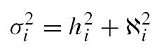
Regarding the variance of the data of model (1), it could be divided into common and unique factors, as can be observed in Eq. (3).

(3)

where var(Y_i) is the variance of the random Y_i observations; the variance of c _i refers to the common variance or communality being researched; and the variance of e _i is the sole or specific variance. The previous equation could also be represented as:

(4)

where the first term is the sum of the effects of the factors and the second is the effect of the disturbance. Calling for the sum of the effects of the factors as:

(5)

where hi2 is the common variance or communality.

Methodology of the confirmatory factor analysis. There are various alternatives to dealing with the model provided in (1) , however, the most common is related to the method of extraction by main components for the creation of composite indicators derived from conceptual models (^{OECD & JRC, 2008}). The general methodology for the analysis is the following: (1) Standardize the original variables, formally done with a transformation of the standard normal distribution with a median of zero and a variance of one through equation 6, due to these being expressed in different units of measurement (^{Espejo Benítez & Hidalgo Pérez, 2011}; ^{Gutiérrez Pulido & Gama Hernández, 2010}; ^{OECD & JRC, 2008}).

(6)

where Z_ij is the standardized variable j with a median of zero and a variance of one of the observation entity i; Y_ij represents each variable j of the observation entity i; Y_j represents the arithmetic median of the values of variable j; S_j represents the standard deviation of variable j.

(2) Obtain the variances of the standardized original variables (Y_ij) with a median of zero and a variance of one, the new variable obtained from this transformation is represented by (Z_ij), which is known as the standardized correlation matrix¹(^{De la Garza García, Morales Serrano, & González Cavazos, 2013}); (3) Through Bartlett's test of sphericity contrast and the Kaiser-Meyer-Olkin measure of sampling adequacy, the degree of general correlation, the partial correlation between variables, and the advantage of the factor analysis were determined for the proposed analysis. With Eq. (7), the values of Bartlett's ji squared were obtained and with Eq. (8), the general measurement of sampling adequacy (MSA_g ) is obtained, which could be extended to the individual variables (MSA _j ) using Eq. (9) to exclude those found to be unacceptable (also identified by values below 0.5 in the main diagonal of the anti-image correlation matrix) (^{De la Garza García et al., 2013}; ^{Hair, Anderson, Tatham, & Black, 1999}).

(7)

where XC2 is the calculated ji squared;nis the number of data;mis the number of variables; |R| is the determinant of the correlation matrix, which ranges between 0 and 1, that is 0≤|R|≤1, a value of 1 indicates that it is an identity matrix.²

(8)

where theMSA _g index is the measure of adequacy of the general sampling delimited between 0 and 1, the acceptable beingMSA _g ≥0.5; and rij(p)2 is the partial correlation coefficient between (Z_i,Z_j) eliminating the influence of the rest of the variables.

(9)

where theMSA _j index is the measure of individual adequacy delimited between 0 and 1, the acceptable beingMSA _j ≥0.5; and rij(p)2 is the partial correlation coefficient between (Z_i,Z_j) eliminating the influence of the rest of the variables.

(4) The individual values and vectors are calculated using Eqs. (10) and (11). Eq. (11) originates the orthogonal matrix for the transformation, renamed L^ (^{De la Garza García et al., 2013}; ^{Peña, 2002}; ^{Pla, 1986}; ^{Timm, 2002}).

(10)

(11)

where Ris the standardized correlation matrix with a (p×p) dimension; λ is a scalar whose lambda values are identified, and are denominated individual values (eigenvalues); I is the identity matrix; L is a non-zero, dimension vector (p× 1) denominated an individual value (eigenvector).

(5) Determine the optimal number of factors, addressing the following three criteria: (a) scree test which is a sedimentation graphic between the number of factors and the eigenvalues obtained from Eq. (10). A variant or option for this criterion is the use of the eigenvalue ≥ 1; (b) multiple linear correlation percentage of each variable with the factors of communality≥ 60%, according to ^{Hair et al. (1999}, p. 93); (c) the accumulated explained variance percentage (PVEA) ≥ 60%, through Eq. (12) (^{De la Garza García et al., 2013}; ^{Espejo Benítez & Hidalgo Pérez, 2011}; ^{Hair et al., 1999}; ^{OECD & JRC, 2008}; ^{Timm, 2002}).

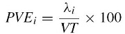(12)

where PVE _i is the percentage of the individual explained variation of factor ith; λ₁ is the eigenvalue of the ith observation; VT is the total variation (or number of variables).

(6) Test the proposed conceptual model.

(7) Carry out an orthogonal rotation of the factor matrix following the varimax rotation method³ that simplifies the visual identification of variable groups, through the loads of the determined optimal factors (^{De la Garza García et al., 2013}; ^{Hair et al., 1999}).

(8)Construction of a competitiveness or codification translator for the CM3L. A joint interpretation of the first two components is carried out based on the loads of the eigenvector of the tested conceptual model, that is, with the interpretation of the first two components that ensure at least a 60% explained variance according to the third criterion of those mentioned in the section on the optimal selection of factors, thus, choosing the loads of the factors (eigenvectors) that multiply each of the standardized variables with Eq. (6) of each entity (^{OECD & JRC, 2008}).

The construction of both the individual ranking of the common determinant factors and the global ranking is done as previously indicated in this step. However, for the easy interpretation of these indexes, equation 13 is used to order the codified data into a zero to one-hundred scale (^{OECD & JRC, 2008}).

(13)

where I_ij is the value of indicator I in the 0-100 scale for entity j; IN_ij is the value of indicator I for entity j; min_j (X_i) represents the lowest indicator from entity j; and max_j(x_i) represents the largest indicator of entity j.

Results

As previously mentioned, based on the empirical evidence of related investigations, and with the support of the statistic program SPSS 17.0 and Minitab 17.0, it was possible to identify the reduction of the 35 initial variables into 6 common factors that provide a 93.675% total explained variance, utilizing in said analysis the criterion of eigenvalue⁴≥ 1 in its standardized variables, as shown in Table 2. This represents both the non-rotated components matrix as well as the rotated components matrix. The six common factors previously mentioned were also used as support to elaborate Tables A1, A2 and A3.

Table 2 Total explained variance and determination of the dimension of the common factors. 

Extraction method: Analysis of the main components.

Source: Own elaboration.

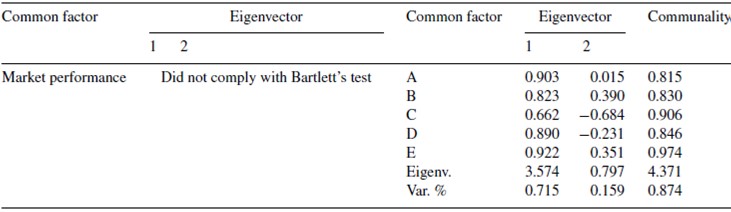
To explain the existing relation between the variables of the determinant factors and the competitiveness of the entities, that is, the existence of the degree of interrelation between the groups of variables, it is necessary to prove the degree of correlation of the defined variables with each common factor.Bartlett's test of sphericity and the adequacy measurement of the Kaiser-Meyer-Olkin sampleprovide the degree of adequacy of the factor analysis.

Table 3 shows the results, demonstrating that both tests determine that the factor analysis is adequate to study the interrelations between the variables of each common factor, except for the labor market performance determinant, due to the fact that its level of significance is too low (0.747). This is the result of proving the absence of significant correlations between the variables defined in this factor. In other words, it proves the null hypothesis that states that the determinant of the correlation matrix adjusts to the identity. Therefore, the labor market performance determinant should not be used in the factor analysis. On the other hand, the knowledge-based economy determinant was accepted with 10 degrees of freedom, due to having delimited one of the variables (candidates) for having aMSA _j value < 0.5, meaning it presented a rather low partial correlation index with regard to the group of variables in said determinant.

Table 3 Kaiser-Meyer-Olkin and Bartlett's test. 

Source: Own elaboration.

From the system of Eq. (1) and Eqs. (10) and (11), the eigenvectors corresponding to the weights of the standardized original variables used to estimate each individual latent variable (or individual indicator) are obtained; and with the ensemble of these latent variables, the eigenvectors are obtained to estimate the global latent variable. The summarized results are shown in Table A4 for the set of said variables.

The above results demonstrate the hypothesis proposed in this work regarding the sustainment of the design of the CM3L based on the review of the literature, validity and the statistic reliability that are summarized in Tables 2, 3 and Table A4. Furthermore, Figure 1 shows the CM3L model, which presents the interrelations between the variables of the determinant factors and the competitiveness of the entities. The data in parentheses refer to the accumulated total explained variation of the first common factor for each determinant, calculated using Eq. (12) from Table A4; the others refer to the datum that relates to the multiple linear correlation coefficient of each determinant in the ensemble of the two factors, which explain 87.4% of the accumulated VT calculated with Eq. (5); the other datum refers to thepvalue in the Bartlett test, which is shown in Table 3.

Even though the market performance determinant was not considered in the analysis, as no significant correlation was found between the variables considered in the study, this does not mean that said determinant is not important, given that there are other variables that could be considered, such as: total exports, total imports, incoming foreign direct investment (FDI), outgoing FDI, percentage share in global FDI arrivals—with these being the variables most cited by the main authors such as ^{Porter (2008)}, among others. However, the data of these variables are not available at the disaggregation level of the municipalities and, therefore, it was not possible to evaluate their impact in the conceptual model.

To characterize the competitiveness of the entities, we proceeded to step eight of the methodology. Thus, the ranking translated to the corresponding position of each of the eleven entities is shown in both Table 4 and Fig. 2.

Table 4 Competitiveness indicators, 2010. 

Name of the determinant:

A. Economic performance.

B. Infrastructure and ICTs.

C. Basic education and healthcare.

D. Qualified human capital.

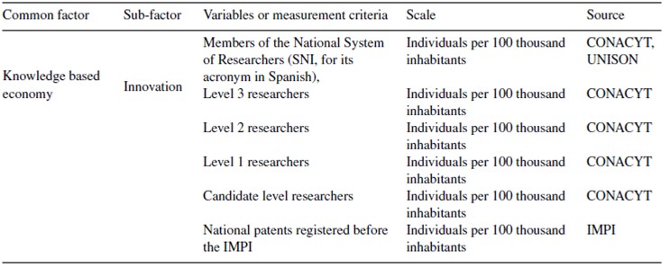
E. Knowledge based economy.

Source: Own elaboration.

Fig. 2 Standardized global line graph for the entities, 2010. 

As pointed out by ^{Garza (2010)}, it is worth noting that the achieved competitiveness ranking of the entities is very similar if only the economic performance determinant is taken into consideration. This is due to this determinant presenting a high composite (or global) multiple linear correlation or Pearson correlation. However, in the case of this study, the interpretation of the global ranking is more complete as it includes the information of the set of competitiveness determinant factors.

Conclusions

Although the concept of competitiveness is very complex, there is consensus regarding said term when it is used at the micro and meso levels. However, at the macro level the concept lends itself to debate by referring to the “competitiveness of nations”. Nevertheless, as previously mentioned, there is consensus between the classical and business schools when the concept relates to the internal productivity of the country, but not with respect to other countries. In this manner, this CM3L model has been developed, among other methods, as a tool for the State policy-makers, decision-makers of the business sector, and academics and researchers interested in measuring, knowing, or explaining the geographical competitiveness of the country, the state, or the municipalities, and to identify what factors need improvement and what variables of the determinant factors have contributed the most to the success of its competitiveness.

The CM3L conceptual model was developed by establishing causality through theoretical justification in other models. With the support of empirical data, 6 competitiveness performance determinants were identified, which were in turn appointed as factors: (1) economic performance, (2) market performance, (3) infrastructure and ICTs, (4) basic education and healthcare, (5) qualified human capital, and (6) knowledge based economy. Furthermore, for each of these factors, sub-factors and variables were identified. These measure the six determinant factors of competitiveness. The sub-factors comprise a second level and the variables a third level of disaggregation, both for the information inputs as well as for their analysis.

The empirical application of the CM3L model shows that upon verification, the hypothesis for 5 determinant factors that influence on the competitiveness of the entities was proven. These are: economic performance, infrastructure and ICTs, basic education and healthcare, qualified human capital, and knowledge based economy. Regarding the labor market performance determinant, it was found that it was not significant due to the variables not being sufficiently correlated, which means that said variables have had a plausible relation or rather that in this type of analysis where the perspective of time (more than a year) cannot be distinguished; with said variables, causality cannot be proven. This does not mean that this factor ought to be eliminated from the conceptual model, but that this dimension needs to be proven using other disaggregated variables at the municipal level including the perspective of time.

The results of the CM3L empirical model shown in Figure 2, illustrate that the municipality of Hermosillo is the most competitive in the country, in the State of Sonora, and among the rest of the municipalities. On the other hand, it was found that the municipality of Cajeme, the State of Sonora, and the whole country are at the same medium stage of competitive development; whereas the municipalities of Guaymas, Nogales, Navojoa, Puerto Peñasco, Caborca, San Luis Río Colorado and Agua Prieta are at a low competitiveness level. The findings coincide with the results reported by the IMCO in 2010, in that they first identify Hermosillo as having the highest competitiveness (in the adequate classification); however, the results diverge when they identify Obregón city (or Cajeme) and Guaymas at the same stage of development, located above the competitiveness average, and the rest of the municipalities are not taken into consideration in their analysis.

Finally, a second stage of this investigation emerges as a conclusive result of this first work. The aforementioned stage corresponds to the identification of competitiveness in the 72 municipalities of the State of Sonora, making said identification comparable in time.

REFERENCES

Anuario estadístico y geográfico de Sonora, INEGI (2013) [consultado 13 Oct 2014]. Disponible en: Disponible en: http://www3.inegi.org.mx/sistemas/biblioteca/ficha.aspx?upc=702825065324 [ Links ]
Artal, A., Castillo, J. y Requena, F. (2006). Ventaja comparativa, dotaciones factoriales y comercio de las regiones españolas con la Unión Europea. Investigaciones Regionales, 8, 85-104. [ Links ]
Artal-Tur, A., Llano-Verduras, C. y Requena-Silvente, F. (2009). Factor productivity differences and missing trade problems in a regional HOV model. Regional Science, 89(4), 759-776. [ Links ]
Becerril Torres, O. U., Alvarez Ayuso, I. C., del Moral Barrera, L. E. y Vergara González, R. (2009). Indicador de infraestructura productivas por entidad federativa en México, 1970-2003. Gestión y Política Pública, 12(2), 379-439. [ Links ]
Benzaquen, J., del Carpio, L. A., Zegarra, L. A. y Valdivia, C. A. (2010). Un índice regional de competitividad para un país. CEPAL, 102, 69-86. [ Links ]
Bracamonte Sierra, A. (2011). Economía basada en el conocimiento. Hermosillo: El Colegio de Sonora. [ Links ]
Castro-Gonzáles, S., Peña-Vinces, J., Ruiz-Torres, A. J. y Sosa, J. C. (2014). Estudio intrapaíses de la competitividad global desde el enfoque del doble diamante para Puerto Rico, Costa Rica y Singapur. Investigaciones Europeas de Dirección y Economía de la Empresa, 20(3), 122-130. [ Links ]
Cho, D. S. (1994). A dynamic approach to international competitiveness: The case of Korea. Journal of Far Eastern Business, 1(1), 17-36. [ Links ]
Cho, D.-S. y Moon, H.-C. (2005). National competitiveness: Implications for different groups and strategies. International Journal of Global Busiess and Competitiveness, 1(1), 1-11. [ Links ]
Cho, D.-S. y Moon, H.-C. (2013). From Adam Smith to Michael Porter: Evolution of competitiveness theory. Singapore: World Scientific. [ Links ]
Cho, D.-S., Moon, H.-C. y Kim, M.-Y. (2009). Does one size fit all? A dual double diamond approach to country-specific advantages. Asian Business & Management, 8(1), 83-102. [ Links ]
CONAPO. (2010). Índice de marginación por entidad federativa y municipio. México, D.F.: Consejo Nacional de Población. [ Links ]
De la Garza García, J., Morales Serrano, B. N. y González Cavazos, B. A. (2013). Análisis Estadístico Multivariante: un enfoque teórico práctico (1.a ed.). México: McGrawHill. [ Links ]
Dunning, J. H. (2003). The role of foreign direct investment in upgrading China’s competitiveness. Journal of International Business and Economy, 4(1), 1-13. [ Links ]
EGAP. (2010). La Competitividad de los Estados Mexicanos. Monterrey: Tecnológico de Monterrey. [ Links ]
Espejo Benítez, J. M. y Hidalgo Pérez, M. A. (2011). Un indicador de competitividad para las provincias españolas. Revista de Estudios Regionales, 92, 43-84. [ Links ]
Garza, G. (2010). Competitividad de las metrópolis mexicanas en el ámbito nacional, latinoamericano y mundial. Estudios Demográficos y Urbanos, 25(3), 513-588. [ Links ]
Gutiérrez Pulido, H. y Gama Hernández, V. (2010). Limitantes de los índices de marginación de Conapo y propuesta para evaluar la marginación municipal en México. Papeles de Población, 16(66), 227-257. [ Links ]
Hair, J. F., Anderson, R. E., Tatham, R. L. y Black, W. C. (1999). Análisis Multivariante (5.a ed.). Madrid: Prentice Hall Iberia. [ Links ]
Heckscher, E. F. (1949) (orig. pub. 1919). The effect of foreign trade on the distribution of income. En S.E. Howard y L.A. Metzler (eds.), Readings in the Theory of International Trade. Homewood: Irwin. [ Links ]
Hergnyan, M., Gabrielyan, G. y Makaryan, A. (2008). Yarevan, Armenia: Economy and Values Research Center. National Competitiveness Report of Armenia, 13. [ Links ]
Hernández Sampieri, R., Fernández Collado, C. y Baptista Lucio, P. (2010). Metodología de la investigación (5.a ed.). Perú: McGraw-Hill. [ Links ]
Hidalgo Capitán, A. L. (1998). El pensamiento económico sobre desarrollo. De los Mercantilistas al PNUD. Huelva: Universidad de Huelva. [ Links ]
IMCO (2007). Competitividad Urbana 2007. México: Instituto Mexicano para la Competitividad A.C. [ Links ]
IMCO (2014). Índice de Competitividad Estatal 2014. México: Instituto Mexicano para la Competitividad A.C. [ Links ]
IMD (2014). IMD World Competitiveness Yearbook [consultado 30 Sep 2014]. Disponible en: Disponible en: http://www.imd.org/wcc/wcc-partner/#tab=2 [ Links ]
Jones, R. W. (2011). Sense and Surprise in Competitive Trade Theory. Economic Inquiry, 49(1), 1-12. [ Links ]
Juozapaviciene, A. y Eizentas, V. (2010). Lithuania exports in the framework of Heckscher-Ohlin International Trade Theory. Economics and Management, 15, 86-92. [ Links ]
Krugman,P.R. (1979). Increasing returns, monopolistic competition and international trade. Journal of International Economics, 9, 469-479. [ Links ]
Krugman, P. (1994). Competitiveness: A dangerous obsession. Foreign Affairs, 73(2), 28-44. [ Links ]
Lall, S. (2001). Competitiveness indices and developing countries: An economic evaluation of the global competitiveness report. World Development, 29(9), 1501-1525. [ Links ]
Lombana, J. y Rozas Gutiérrez, S. (2009). Marco analítico de la competitividad fundamentos para el estudio de la competitividad regional. Pensamiento y Gestión, 26, 1-38. [ Links ]
Moon, H. C., Rugman, A. M. y Verbeke, A. (1998). A generalized double diamond approach to the global competitiveness of Korea and Singapore. International Business Review, 7(2), 135-150. [ Links ]
Nyahoho, E. (2010). Determinants of comparative advantage in the international trade of services: An empirical study of the Hecksher-Ohlin Approach. Global Economy Journal, 10(1), 1-22. [ Links ]
OECD & JRC (2008). Handbook on Constructing Composite Indicators Methodology and User Guide. Château de la Muette, Paris, France: OECD Publications. [ Links ]
Peña, D. (2002). Análisis de datos multivariantes. Madrid: Mc Graw Hill. [ Links ]
Pla, L. E. (1986). Análisis Multivariado: Método de componentes principales (1.a ed). Coro, Falcon, Venezuela: The General Secretariat of the Organization of American States Washington, D.C. [ Links ]
Porter, M. E. (1990). The Competitive Advantage of Nations. Harvard Business Review, 73-93. [ Links ]
Porter, M. E. (2008). On competitition: updated and expanded edition. Boston: Harvard Business School Publishing Corporation. [ Links ]
Quijano Vega, G. A. (2007). La importancia de la competitividad económica en el desarrollo de los municipios del Estado de Sonora, México. Observatorio de la Economía Latinoamericana, 77(16). [ Links ]
Ramos Ramos, R. (2001). Modelo de evaluación de la competitividad internacional: una aplicación empírica al caso de las Islas Canarias [tesis en opción al grado de Doctor en Ciencias Económicas]. Las Palmas de Gran Canaria, España: Universidad de Las Palmas de Gran Canaria. [ Links ]
Ricardo, D. (1971) (orig. pub. 1817). The Principles of Political Economy and Taxation. Baltimore: Penguin. [ Links ]
Romo Murillo, D. y Musik, G. A. (2005). Sobre el concepto de competitividad. Comercio Exterior, 55(3), 200-214. [ Links ]
Rugman, A. M. (1991). Diamond in the rough. Business Quarterly, 55(3), 61-64. [ Links ]
Rugman, A. M. y D´ıCruz, J. R. (1993). The double diamond model of international competitiveness: The Canadian experience. Management International Review, 33, 17-39. [ Links ]
Smith, A. (1937) (orig. pub. 1776). An inquiry into the nature and causes of the wealth of nations. En C.W. Eliot (ed.), The Harvard Classics, New York: P.F. Collier & Son Cororaton. [ Links ]
Timm, N. H. (2002). Applied Multivariate Analysis. New York, NY: Springer. [ Links ]
Travkina, I. y Tvaronaviciené, M. (2010). An investigation into relative competitiveness of international trade: The case of Lithuania. 6th International Scientific Conference. pp. 504-510. Vilnius, Lithuania: Vilnius Gediminas Technical University. [ Links ]
WEF (2014-2015). The Global Competitiveness Report. Geneva: World Economic Forum [ Links ]
Annexes
Table A1 Determinant factors and variables of municipal competitiveness. Part 1.
Source: Own elaboration, taken from the databases.
Table A2 Determinant factors and variables of municipal competitiveness. Part 2.
Table A3 Determinant factors and variables of municipal competitiveness. Part 3.
Table A4 Weights or loads from the latent variables to estimate the global latent variable.
Name given to the determinant or common factor: