


Servicios Personalizados
Revista
Articulo
 texto en
  Inglés (pdf)
 Artículo en XML
 Referencias del artículo
 Enviar artículo por email
Indicadores
-
 Citado por SciELO
 -
 Accesos
Links relacionados
-
 Similares en
SciELO
Similares en
SciELO
Compartir

 Permalink
Contaduría y administración
versión impresa ISSN 0186-1042
Contad. Adm vol.62 no.1 Ciudad de México ene./mar. 2017
https://doi.org/10.1016/j.cya.2016.10.001
Articles
Economic integration, economic crises and economic cycles in Mexico
a El Colegio de la Frontera Norte, México
This article analyzes the peculiarity of the dynamics of economic fluctuations of the Mexican economy, within the framework of its integration with the US and Canada; the article demonstrates how the Mexican economy make endogenous the macroeconomic crises from the USA (2001 and 2007), and how the business cycles of both countries became more aligned to each other.
Based on the heterodox economic theory of crises and cycles, we check the "empirical law of economic dynamics" of the Mexican capitalist system according to the logic of the multiplier-accelerator theory that allowed us to study the dynamics of business cycles for the period of the study (1993-2013). To do this, we construct and estimate a stationary VAR model and utilize the Granger causality tests and quarterly data.
Keywords: Economic integration; NAFTA; Crisis; Business cycles; Growth
JEL classification: C32; E32; F02
En este artículo se analiza la peculiaridad de la dinámica de las fluctuaciones económicas de la economía mexicana en el marco de su integración con Estados Unidos y Canadá, y se demuestra cómo la economía mexicana endogeneizó las crisis macroeconómicas provenientes de Estados Unidos (2001 y 2007) y cómo los ciclos económicos de ambos países se fueron alineando. Con base en la teoría económica heterodoxa de las crisis y los ciclos verificamos la «ley empírica de la dinámica económica» del sistema capitalista mexicano según la lógica de la teoría del acelerador-multiplicador que nos permitió estudiar la dinámica de las fluctuaciones para el período de estudio (1993-2013). Para ello, construimos y estimamos un modelo VAR estacionario y utilizamos las pruebas de causalidad a la Granger y datos trimestrales.
Palabras clave: Integración económica; TLCAN; Crisis; Ciclos económicos; Crecimiento
Códigos JEL: C32; E32; F02
Introduction
With the signing of the North American Free Trade Agreement (NAFTA), a very important phase in the history of the Mexican economy began. This phase has been thoroughly analyzed, with regard to its impact on commerce, investments, and employment, among other important macroeconomic variables. Nevertheless, we consider it necessary to study the macroeconomic implications of this economic integration period, in terms of the dynamics of the economic cycles and their relation to the economic crises that have arose since 1994 and up to present day; considering that the macroeconomic short-term stabilization policies and the series of structural reforms implemented have tended to modify the dynamic of the cycles and the behavior of economic crises.
Particularly, during the period of the NAFTA, the policies of public spending and monetary control turned into powerful macroeconomic instruments to permanently adjust to the aggregate demand, becoming pro-cyclical policies. That is why the macroeconomic dominant features of the period were: the deceleration, economic stagnation, the presence of more unstable economic cycles, and more acute macroeconomic crises. In this work, we analyze and confirm how after the crisis of 1994, the Mexican economy endogenized the macroeconomic crises of the USA (2001 and 2007), and how the cycles of both countries aligned as a result of the growing integration of the Mexican economy to that of the American economy. This way, a new macroeconomic instability stage arose in the history of the country.
This article comprises the following sections: in the first we define the concept of economic cycle and of crisis in a heterodox view; in the second we analyze the main macroeconomic characteristics of the period, the behavior and the morphology of the cycles and of the economic crises of Mexico during the period being studied; in the third we study the co-movements of the supply and demand aggregated components with regard to the Mexican economic cycle and their synchronization level with regard to the American cycle; and in the fourth we present the econometric results of the VAR model that we applied in order to simulate the effects of the random shocks on the Mexican economic system; and finally, we present our conclusions.
Theoretical framework: crisis and growth cycles
The main heterodox economic theories that have studied the relation between the macroeconomic crises and the economic cycles establish that the cycles and the crises are explained by the dynamic of capital accumulation and of effective demand. According to this, the general economic crises are closely linked to the dynamic of the economic cycle; the crises mark the end of an expansion phase and the start of another cycle.1 In this sense, Marx (1965) argues that the modern economic cycles are the result of a capitalist production system and reference the dynamic and reproduction of the social or global capital as a finite set of individual capitals, the movements of which determine the dynamic of the capitalist economy in its entirety.2 Thus, for Marx (1965), the capitalist economies follow a dynamic that is analog to that of the "celestial bodies which, once they have been launched into orbit they follow it for an indefinite amount of time, the same happens with the social production, once it is launched, this alternative expansion and contraction movement will repeat it due to mechanical need. The effects become causes and the incidents, first irregular and accidental, affect normal periodicity more and more." (Marx, 1965; p.1149-1150). The law that governs on the long term is more dynamic, it is the law of the fall trend of the rate of profit. From Marx's perspective, the crises arise when there is a turning point3; this is when the overproduction of merchandize has no market,4 it is at this point that the expansion phase of the capitalist production system ends.5 So that the plethora of individual capitals produced under the form of merchant capital that could not be sold, result on a general crisis (M kt ' > D kt '), in the form of an effective demand crisis with the corresponding unemployment. Which then ends an entire optimism phase in the financial market (D-D').6 After the crisis, a period of economic contraction begins, a period of destruction and of the emergence of new individual capitals, with which the beginning of a new expansion phase that corresponds to a new economic cycle is prepared. In each crisis, there is a massive destruction and fusion of individual capitals (concentration and centralization of capitals), in particular, the financial or fictitious capital is devalued (D kt ’ > D kt ’’). From a more complex perspective, the crises arise as a result of the sudden fall of the rate of profit and the presence of an enormous amount of profit that cannot be accomplished (Marx, 1965; pp. 1149-1150). "In the course of the cycle, businesses go through successive stages of depression, medium animation, precipitation and crises. "Even though the capital investment periods differ from one another, the crisis constitutes the starting point for new investments, it constitutes a new material base for the next cycle of capital rotations." (Marx, 1965; p. 614). Marx proposes that the Juglar7 cycles have an approximate duration of ten years, but this figure is not constant because its duration depends on the technical progress (Marx, 1965; pp. 1149-1150), which reduces the duration time of the fixed capital and thus the temporality of the cycle. Therefore, technical progress is a factor that tends to reduce the duration of the cycle (Marx, 1965; p. 614).
In the same theoretical perspective, Rudolf Hilferding (1971) observes that there is an empirical law of the dynamic of the capitalist system, according to which, the capitalist mode of production is bound by a circle of prosperity and depression, where the general crises result from the transition of one to the other (Rudolf Hilferding, 1961; p. 270), "at any given moment during prosperity, there will be stagnation in a series of branches of production: consequently, the prices drop. Stagnation and the reduction of prices expand; the production is limited and the situation lasts for more or less time. The prices and the benefits are low and little by little the production begins to expand, the prices increase as well as the benefits. The volume of production is greater than ever until the situation varies again. The periodic repetition of this process presents the issue of what causes it, which has to be investigated through the analysis of the capitalist production mechanism." (Rudolf Hilferding, 1961; p. 270). Another factor that causes the explosion of the crises is the imbalance that is unchained between the productive branches of the capitalist production system due to the anarchic nature of the capitalist production and the lack of proportionality between them, which is expressed in the disruption of the law price.
Joseph Schumpeter (1935) in turn, believes that the dynamic of the capitalist development is neither uniform nor linear, but that it fluctuates as it maintains typical increases and decreases. These increases and decreases are characterized by the presence of turning points or crises that mark the rupture between both phases. For Schumpeter (1935), the crises are the passage of prosperity to depression and they give rise to the emergence of abnormal events (panic, bankruptcies, ruptures, etc.). Both for Juglar and for Schumpeter the only cause of depression is prosperity, depression is the reaction of the capitalist economic system before the economic boom that preceded it.
In turn, the explanation of Keynes (2005) on the general crises and the economic cycle, is situated on the perspective of effective demand (M kt ’ > D kt ’), according to him, the macroeconomic crises are the result of the sudden fall of the marginal efficiency of the capital, and they represent the sudden and violent change of the macroeconomic situation in a country. For Keynes (2005), in the last stages of the economic boom the expectations with regard to future profits are too optimistic and there is an increased abundancy of the capital goods, a rise of their production costs and of the interest rates. This is why macroeconomic crises appear at the end of an ascending prosperity phase, and they mark the beginning of a recession and economic depression phase. Keynes (2005) therefore considers that in the last stages of the economic boom the expectations with regard to future profits are too optimistic. The financial markets (D kt - D kt ’ - D kt ’’ - D kt ’’’...) are subject to: (i) the influence of the buyers that ignore what they buy, (ii) the speculators that are solely interested in the changes of opinion regarding the stock-market, more than on the rational estimation of the future profits of the capital goods. The stock-market courses drop suddenly and catastrophically when reality crashes on an overvalued or optimistic market, panic ensues and then bankruptcy, as well as the massive destruction of the financial capital (D kt ’ > D kt ’’ ), a situation also described by Marx.
We can observe that for Marx, Hilferding, Schumpeter and Keynes, the macroeconomic crises are necessary moments of the capitalist economic dynamic, represented by economic cycles; this is why they have an endogenous nature and are determined by investment and the accumulation of capital.
Macroeconomic behavior, crises and the morphology of the Mexican economic cycles
From the perspectives of Marx (1965), Hilferding (1971) and Keynes (2005), the cycles and crises are closely related. According to these authors there is an "empirical law of the economic dynamic" that rules the capitalist system, according to which, the development of the economic system follows an irregular cyclical empirical trajectory, with high-crisis-low phases; the existence of which we will empirically verify for the case of Mexico.
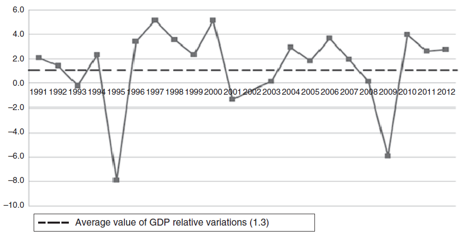
During the period (1994-2013) the first and second generation structural reforms were implemented derived from the Washington Consensus, and starting on 1994, a regime of Flexible Change predominated. Unemployment was at 3.8% on average, the GDP grew at an average rate of 2.6%, exports had a participation of about 27.95%, the average participation of imports on the GDP was of 29.39%, and of investments of 23%. The per-capita GDP of the Mexican economy grew at an average rate of 1.3% (Table 1, Fig. 1); according to Hausmann's rule, as this indicator grew under 2.4%, the economy may be listed as stagnant.
Table 1 Macroeconomic behavior of the Mexican economy: 1993-2012.
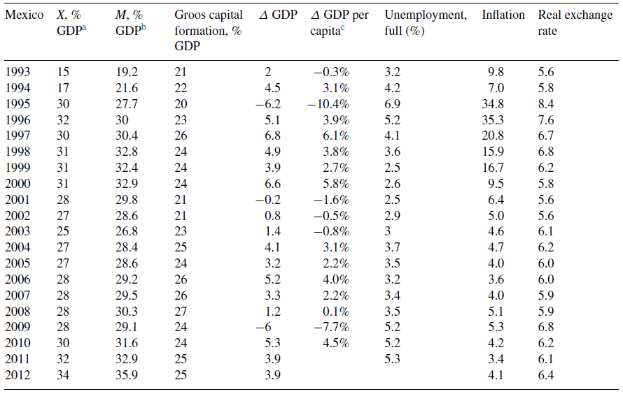
a Exports of goods and services.
b Imports of goods and services.
c PPP Converted GDP Per Capita (Laspeyres), derived from growth rates of c, g, i, at 2005 constant prices.
Source: INEGI.
Another macroeconomic feature is that a low inflation rate remained during the entire period, it was a rate of one digit due to the fact that the government maintained a restrictive inflationary control monetary policy, using restrictive monetary and fiscal policies (see Table 1 and Fig. 1). The crisis of 1994 proved that it was impossible to keep stable the exchange rate, the Pegged Exchange Rates8 policy to control inflation based on the exchange rate as the nominal anchor and applied since 1988, failed. Therefore, in 1999 an Inflation targeting-IT strategy was adopted, this was done in order to achieve two objectives: the decrease in the level and variability of the inflation, and a high output stability. However, this strategy demonstrated, in Mexico and other countries, that it was unable to simultaneously stabilize the output and inflation, and achieve low unemployment rates or high economic growth rates (Brito & Brianne, 2010). This monetary policy (IT) also favored the appreciation of the real exchange rate.
After having implemented the institutional reforms in Mexico, which led to the autonomy of the Central Bank and to a monetary policy (IT) that reduced inflation, a FFIT regime of the Inflation Targeting Lite (LITE-IT) began.9 This policy, along with a final restrictive policy brought along with it a slow growth (Fig. 1) and the control of inflation, which was reduced to one digit.
In this manner, the implementation of these macroeconomic policies prompted the restriction of the aggregated demand and the appreciation of the exchange rate. On the other hand, the appreciation of the exchange rate, favoring the import of consumables and goods at an inferior cost, contributed to the disruption of the productive capacities of the Mexican economy, which led to its deceleration.10
During the entire period of validity of the NAFTA, the main objectives of the fiscal policy have been to maintain a balanced budget and an adjusted aggregated demand, even in macroeconomic periods without inflation. Thus, public spending, far from turning into an anti-cyclical policy instrument, became a pro-cyclical instrument,11 which tends to accentuate the effects of the macroeconomic crises. The dynamic of the economic cycles has become more unstable, the recovery has weakened and there have been expansion phases of the cycles that are above the potential GDP, which emphasizes the deceleration of the economy.
We will now analyze, for the case of Mexico during the period between 1993.1 and 2013.3 the "empirical law of the economic dynamic" as is defined by Hilferding. We will study the growth cycles that we have defined as the relative highs and lows of the GDP with regard to its tendency.
Following this methodology, a series of growth cycles in the Mexican economy were identified for the study period of 1993.1 and 2013.3 (Fig. 2 and Table 2), which together help to shape the trajectory of their dynamic. It is observed that the phases of these growth cycles of the GDP fluctuate around the tendency line or potential GDP that is represented by the horizontal line with the coordinate 100. Fig. 2 shows the behavior of the economic cycles of the Mexican economy and the first thing that can be proven is that they are not the same, and that each one varies in a different manner, both in duration and intensity or range. The gray bands in the figure show the recessions of the United States of America (USA), which coincide with the recessions of the Mexican economy in the years 2001-2002 and 2007-2009. A tendency toward the endogenization of the American crises by the Mexican economy can be observed.
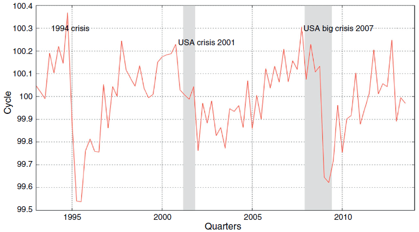
Source: INEGI and National Bureau of Economic Research (NBER). Own elaboration.
Figure 2 Growth cycles in the NAFTA age.

The presence of four cycles and three major macroeconomic crises situated at the peaks of the cycles that correspond to the years 1994:4, 2000:3 and 2007:4 is confirmed (see Table 2). The crisis of 1994 was fundamentally caused by internal macroeconomic variables, while the crises of 2000:3 and of 2007:4 developed as a consequence of the American crises. In the era of the NAFTA, a tendency toward a greater integration of the Mexican economic cycle with the American cycle can be observed. Furthermore, the economic cycles and their corresponding crises have become more volatile and dependent on the American economy. The macroeconomic crises tend to align with the American crises of 2001-2002 and of 2007-2010 and the cycles had an average duration of 6.5 years.
We identified four cycles during the study period, the characteristics of which are the following:
First cycle: marked by the crisis of 1994, named the first globalization crisis, with an internal origin, and which was the result of the potentially existing contradictions between: the anti-inflationary "heterodox" policy of stabilization, the growth strategy aimed at exports, and the opening for the globalization of the monetary and financial national system. The crisis was the direct consequence of "the abundancy of external capital inputs, resulting of the structural reforms and the international financial juncture" (Calderón & Caire, 2012), which brought along a boom phase for the Mexican economy, and in turn generated an increased difficulty for financing in the adjustment between saving and investment. The financial crisis of 1994-1995 was caused by the applied anti-inflationary measures based on the fixed exchange rate as a nominal anchor, the monetary sterilization policy and a political clash that reduced the optimism on the period. The declining phase of the cycle lasted 9 months, though the range of the descent was more profound (0.71). The deceleration phase (-0.44) was broader than the acceleration phase (0.27).
Second cycle: marked by the macroeconomic crisis of 2000.3-2001, this 8-year cycle is characterized by its ascension phase (0.65), which was superior to the descent phase (0.45), and an acceleration phase (0.21) superior to the contraction phase (-0.176). The expansion was determined by the strong expansion of the USA in the nineties, which ended the crisis at the start of 2001, moment in which the global economy showed a simultaneous deceleration in the United States, Japan and Europe, which led to a severe contraction of the trade flows of the international market. This deterioration of global growth negatively impacted the performance of the Mexican economy, with losses in the levels of private investment, and employment. The Mexican economy slowly recovering after 2002.
Third cycle: marked by the great macroeconomic crisis of 2007.4, this 7.5-year cycle is characterized by having an ascent phase (0.3623) inferior to it is the descent phase (0.45), and an acceleration phase (0.1871) inferior to its contraction phase (-0.26). The expansion was determined by the expansion of the USA after its recession in 2001-2002. A recession that ended with the subprime crisis, a financial crisis of the United States in 2007.
This financial and economic crisis in the United States has been cataloged as the most serious in its category since the great depression of '29 and having had a strong impact on the global economy. In this sense, the crisis tended to reverse the economic expansionist powers of the global market, framed in the dominant ideology of liberalism and of laissez-faire. The financial and economic crisis of the United States was a general crisis of global and international dimensions.
According to its morphology and characteristics of the economic cycle, the crisis was the peak or turning point of the expansionist economic tendencies that inaugurate the emergence of a descent phase, even more so in Industrialized countries. The American economy contracted 0.5 per cent in the third trimester of 2008, which would represent its greatest fall since 2001. In the case of the Mexican economy, its GDP contracted 6% between 2007, 2008 and 2009, and it recovered in 2010 (Table 1).
Fourth cycle: one that has not yet ended, and a macroeconomic crisis that could possibly happen between 2015 and 2016, a cycle that would have an approximate duration of 8-7.5 years. This cycle is characterized by having an ascent phase (0.3663), and an acceleration phase (0.1031).
In general terms, it can be observed that since the crisis of 1994, the Mexican economy has suffered a progressive deceleration tending to go stagnant, this is linked to the growing synchronization of the Mexican economy with the American cycle with regard to the so called globalization. It is observed that the economy progressively endogenized the international crises, and lost its autonomy and its ability to stabilize its national cycle, endogenizing the risk and the international economic uncertainty. Thus, the acceleration phases of the four cycles tended to decrease by 0.27, 0.21, 0.18 and 0.10, respectively, observing a constant tendency toward the deceleration of the dynamic of the Mexican economy between 1993 and 2013. The crises of 2000.3 and 2007.4 of the USA affected the Mexican economy in a significant manner, as it is subject to the American economic cycle, suffering a great impact on the level of its economic activity, with the manufacturing sector as the most affected. In addition to the stock-market contagion derived from the financial crisis, the recession of the United States reduced the flows of foreign investment and remittances that come from said country, with the exports and imports also suffering. Due to this, the level of interdependency of the economic processes of these two countries has been increasing.
Levels of association of the aggregated supply and demand with the economic growth cycles of Mexico
Methodology used
From the start of the economic growth cycles of the Mexican economy between 1993.1 and 2013.3 we are going to determine the level of association or co-movement that exists between these cycles and the components of the aggregated supply and demand of the Mexican economy (Table 3). In order to begin constructing the series of cycles of the real GDP and the associated macroeconomic variables that are present in Table 3, corresponding to the study period of 1993.01-2013.03, we first used trimestral seasonally adjusted macroeconomic series measured in millions of pesos with a 2008 base, same that we proceeded to transform in logarithms; second, we proceeded to separate the tendency of the GDP cycle using the Hodrick-Prescott cycle; and third, we constructed the series from the aforementioned definition.

Degree of association or co-movement of the supply and demand components added with the Mexican growth cycle
Before examining the cyclical structure of the components of the real GDP, it is important to estimate the magnitude of the contribution of each of the macroeconomic series to the economic fluctuations. To this end, we calculated in Table 4 a series of relevant statistics that measure this regard. Here, the first line provides us with the relative magnitude of the macroeconomic aggregates of supply and demand as a percentage of the GDP.
Table 4 Average values from 1993.1 to 2013.3.
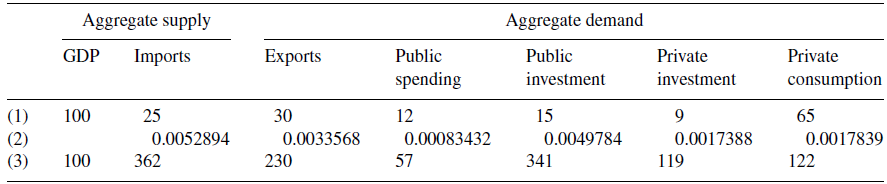
(1) Average of the series divided by the average GDP, percentage.
(2) Standard deviation of the series without trend divided by the mean of the series
(3) Standard deviation of the series divided by the standard deviation of the GDP
Source: Own elaboration based on INEGI data.
During the analysis period, from 1993.1 to 2013.3, we observed that private consumption is the most relevant variable with 65%, whereas private investment is the one with the least dynamic importance in the GDP with only 9%.
The second line presents information on the fluctuation intensity of each series with regard to their average value, i.e., the degree of volatility with regard to its own average; in general terms, it is very low for all series during the entirety of the study. However, it is observed that the most volatile variable is imports, whereas private consumption, which is the aggregate with the greatest importance, is the least volatile. The third line indicates the degree of volatility of each of the microeconomic variables with regard to the standard deviation of the GDP. Public spending is the least unstable variable, but has a relatively low importance on the GDP with only 12%; the unstable variables are imports with an importance of 25% on the GDP and public investment with an importance of only 15% on the GDP. It is worth noting that private consumption, which determined the dynamic of the GDP for a period, had the highest volatility level. Therefore, any variation in private consumption tends to magnify the cyclical oscillations of the GDP.
We shall now analyze the co-movements of the variables with the growth cycles, studying the degree of correlation (Column 1, Table 5) and the volatility level (Column 2, Table 5) as a means to do so. An important trait of the period is that all variables are pro-cyclical. Private consumption was the variable that, in addition to having the greatest average importance on the GDP throughout the period, was the most correlated with the GDP; furthermore, given that it is a highly volatile variable, it influenced in a determining manner on the oscillations of the economic cycles. Table 5 shows the high degree of correlation that this variable maintains with the cycles of the period (0.9502). Likewise, given that its co-movements are pro-cyclical, they determine at a high level the oscillations of the same. That is to say, ceteris paribus, an expansion of private consumption causes the rise of the cycle and a decrease of the same provokes the contraction of the cycle. In short, during the period there was a high degree of positive correlation between private consumption and the growth cycles, and consequently the co-movements between both variables are highly pro-cyclical. This high correlation is explained in part by the presence of income (remittances, wages, and salaries) highly dependent on circumstances, given that they increase in the expansion stages, and decrease in the contraction stages.
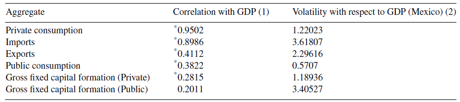
Imports, a variable of the aggregated demand, show a high degree of correlation with the cycles (0.8986), which implies that during the economic expansion stages the import of end products and productive inputs increases, whereas they decrease during the contraction stages. This strong correlation is explained by the growing interdependence with the American economy, and the growing importance that intra-industry commerce has in the external sector of the Mexican economy, derived from the imports of productive inputs and machinery and the consecutive loss of productive capabilities and the deindustrialization of the Mexican economy during the period. During the stage of the NAFTA, the transnationals develop industrial models of shared production and international competence through the differentiation of their products, implementing in the continents and in the country production segments that require low wages and low skilled labor. Whereby Mexico is used as a platform to produce a part of their final product that is sold in the American and international markets. Furthermore, the presence of a stronger exchange rate has favored the growth of the intra-industry commerce.
Exports have a relatively low positive correlation with the cycle (0.4112) in spite of the economic openness and a high volatility. This is explained in part by the fact that exports have not become the driving force of the Mexican economy. This is due to the importance of intra-industry commerce, given that a central component of the exports directed toward the American market are goods assembled or manufactured on national territory. Intra-industry commerce has had to displace inter-industry commerce, which was dominant before the economic openness. This means that free commerce has not favored inter-industry commerce all that much, it has instead favored monopolistic competition and large multinational companies. In fact, the behavior of the exchange rate has favored this type of market structures.
Public consumption maintains a low correlation (0.3822) with the cycle, as well as a stable relation with the same and is pro-cyclical, a reflection of a neoliberal fiscal policy that has tended to intensify the instability of the cycle as a consequence of accentuating the breach between savings and investment. This contrasts with what would be a Keynesian policy of public spending, which follows an anticyclical behavior, focused on reducing unemployment, in order to counteract the effects of crises and economic fluctuations, and which as a fundamental component of effectivedemand compensates the growing gap between savings and investment.
The positive correlation between net investment and the cycle is rather low (0.2815), which indicates that the association level between both variables is extremely reduced in spite of maintaining a positive relation and a low volatility. Private net investment practically does not influence the behavior of the economic cycle; an explanation is that the multiplier-accelerator effect is far too reduced in the framework of a small open economy, with a low level of stock capital and domestic investment and prevalence for foreign investment. Consequently, private investment did not fulfill its role in balancing the market of goods (I-S or M-M’) during the period.
Lastly, public investment does not have any degree of association with the cycle; this is explained by the restrictive fiscal policy, the decrease of expenses in public investment and infrastructure, and the destruction of the productive capabilities of the public economy, all of which is vital for economic growth and acceleration.
Synchronization of Mexico and American economic cycle between 1993.1 and 2013.3
In this section we analyze the degree of synchronization of the Mexican cycle with regard to the American cycle. We use the real GDP at 2008 prices as the identifier of the cycle in Mexico and the non-seasonal GNP at 2009 prices as the identifier of the cycle in the USA.
The GDP cycles of Mexico and the United States are highly synchronized (0.536421) (Table 6). This is due mainly to the high degree of integration of the Mexican economy with the American economy as a result of signing the North American Free Trade Agreement (NAFTA). The major explanatory factors for this are the prevalence for intra-industry commerce between both countries, derived from the fact that the USA is Mexico's major commercial partner12; and that the largest amount of direct foreign investment comes from said country. These factors have strengthened the manufacturing and industrial interdependence between both economies, above all with the implementation of the manufacturing plants in Mexico. Another factor has been the migration influx of Mexicans to the USA, which took place mainly during the 90s, generating a massive flow of remittances toward our country.

Empirical methodology: specification of the model and econometric results of the VAR model
Based on the theory of the accelerator-multiplier model of the cycles, we chose the macroeconomic variables that explain the behavior of the growth cycle of the Mexican economy for the study period of 1993.1 to 2013.1. Based on eight macroeconomic variables represented in Table 1, we constructed and estimated a stationary VAR model in order to analyze the dynamic of the economic cycle. Studying the dynamic of the short-term effects of the random shocks in the cycle, we shall finally carry out the Granger causality tests.
Choosing the macroeconomic variables of the model
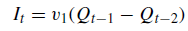
In order to evaluate the short-term effects of the random shocks on the economic growth cycles, we constructed a stationary VAR model whose variables were selected from the theory of the accelerator-multiplier model. According to Harrod (1948), Samuelson (1938), and Kalecky (1935) the imbalances of the markets are what determine the fluctuations or cycles. In these models, the accumulation of capital and investment play a fundamental role, in that the investment has a double nature: on the one hand it is the most volatile variable of the aggregated demand; on the other hand, it is an essential variable for the supply in a closed economy. The dynamic of the imbalances caused by the accumulation of capital is summarized in the multiplier-accelerator model, which provides the most important explanation of the economic cycle. The multiplier-accelerator dynamic lies in the behavior of the investment and imbalances in the goods market, the investment depends on the breach between the anticipated demand and the available production capability, and it is a variable that adjusts to the balance of the goods market. Let us assume that there is a delay of time between the investment and the increase of capital, the net investment is equal to the breach between the stock capital available for the anticipated period (t + 1) and the stock capital available for the period (t). If the coefficient of the capital is constant (v), then the desired capital for the period (t + 1) is proportional to the anticipated demand (k t + 1 = vQ t + 1 ). Therefore, the net investment could be expressed as the breach between the anticipated demand and the available capability, and a proportionality of the anticipated variations of the demand (accelerator model).
 (1)
(1)
Let us extend basic model of Samuelson (1938) by assuming the existence of a small and State open economy, this model of the multiplier-accelerator is susceptible to create a cycle in accordance with the observed evolutions. Therefore, we start from the following macroeconomic identity:
 (2)
(2)
Integral identity (2): commercial balance (X t - M t ), governmental spending G t , the autonomous component of demand A t , private consumption, C t adjusted to the income with the delay of a period:
 (3)
(3)
Private investment is adjusted with the delay of a period to the variations of production, as partner13:
 (4)
(4)
And the behavior relationships of the exports are determined by the behavior of the external income of a large economy Q* t-1 :
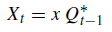 (5)
(5)
And the imports that are going to be determined by the fluctuations of the domestic GDP:
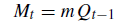 (6)
(6)
Governmental spending is going to be defined as follows:
 (7)
(7)
Added to governmental investment:
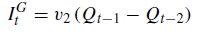 (8)
(8)
Consequently, the total investment is going to be defined as the sum of governmental and private investment:
 (9)
(9)
Solving the model, we would have a second order autoregressive form of the following form:
 (10)
(10)
According to this model (10), the coefficients of private v 1 and governmental v 2 capital determine the magnitude of the oscillations and tend to impulse economic expansion, whereas the imports have the contrary effect, m <0 and c >0 have expansionary effects derived from the multiplier effect in conjunction with exports x > 0.
Variables, data, empirical specification of the VAR model
A stationary econometric VAR model is estimated, using the accelerator-multiplier theory in order to select the endogenous variables that comprise it. This econometric technique allows us to evaluate the impacts derived from the random shocks generated by the changes of these macroeconomic variables (private consumption, public and private investment, the net product of the USA, import and exports) on the economic cycle, for a given analysis period (1993.1-2013.3). Furthermore, we carried out a Granger causality analysis in order to determine which of the considered variables cause, in Granger's sense, random shocks to the cycle. In this manner, we are going to validate as a whole the theoretic explanation of the cycle offered by the accelerator-multiplier model and define its degree of validity for the Mexican case in the period between 1993.1 and 2013. The variables chosen for the estimation of the stationary VAR model are shown in Table 1, have a quarterly frequency, and cover the period between 1993.1 and 2013.3. All the macroeconomic series are non-seasonal and are measured in pesos as per 2008. They were all transformed into logarithms and had their tendency removed from a breakdown of the series, utilizing the Hodrick-Prescott filter.
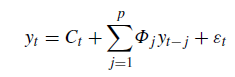
Generally, the autoregressive vectors (VAR (p)) are used to predict the behavior of interrelated systems of temporal series. They are also used to analyze the dynamic generated by the impact of a random shock in any of the variables of the system of variables (called impulse-response-IRF functions). The VAR approach avoids the need to make a distinction a priori between exogenous and endogenous variables from a predetermined theory, this is done by individually treating each endogenous variable in the system as a variable determined by the past values of all the endogenous variables of the same system. The VAR (p) model is mathematically formulated in the following manner:
 (11)
(11)
where ε t is a vector of perturbations without autocorrelation (denominated innovations), with a null average and a matrix of instantaneous co-variances E [ε t ε' t ] = Ω. The residues have a variance and co-variance matrix Ω that by definition is symmetric and, in general, has no restrictions. This system of equations is an autoregressive vector representation (VAR(p)) where φ j , j = 1,..., p are matrices nXn that pick up the dependence of y t about y t-p . According to the relationship, (11)y t is a vector of k endogenous variables, x t is a vector of d exogenous variables, and Φ 1,…, Φ p yΓ t are the matrices of coefficients that are going to be estimated. Now, given the absence of simultaneity in the equation, the technique of minimum ordinary squares is the most adequate to carry out the estimations. In order to select the order of the VAR, that is, to determine the number of delays present, the verisimilitude ratio test and the AIC, among others, are used. From the structure of the VAR(p) model, as determined, the predictions are generated after carrying out a general diagnosis of the estimated models. Once the VAR(p) model has been selected, the answers to the posed economic problems are done as follows: the impulse-response analysis or sensitivity analysis. In this manner we estimate the following stationary VAR(p) Model:
 (12)
(12)
where y t = [Q t , CP t , I p t , I g t , GDP t , GP t , M t , X t ]' is the vector of stationary endogenous variables, C t is the vector of the constants, and e t is the vector of the innovations of the model.
Tests and results
Having estimated a stationary VAR(p) model, we proceed to carry out the unit root test and seasonality test for each of the eight variables to be used in building the VAR(p) model, the results are shown in the Table 7. Here we apply a three-test battery. The first being the ADF test whose null hypothesis lies in the presence of the unitary root, the second being the PP test whose null hypothesis is also the presence of the unitary root; and lastly the KPSS test whose null hypothesis lies in the presence of seasonality. Therefore, if the null hypotheses of the first two tests are rejected, the series are stationary, and if the null hypothesis of the KPSS test is not rejected, the seasonality of the series is confirmed. Given that the variables are stationary, we cannot define a VEC nor find long-term relationships between them, therefore, we proceed to build a stationary VAR(p) based on which we simulate the effects of the random shocks on the dynamic of the cycle (Table 7).
Table 7 Unit root and stationarity tests.
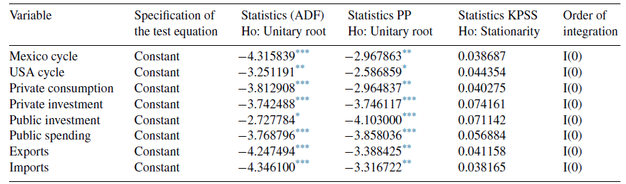
Source: Authors’ own calculations.
* Rejected at 10%.
** Rejected at 5%.
*** Rejected at 10%
Once we have verified that the eight variables are stationary, we move on to the selection of the order of the VAR by determining the number of delays present, for which we apply five information criteria: Akaike (AIC) 1973, Schawars (SC) 1978, Hannan-Quinn LR, FPE, AIC, SC and HQ, which are shown in Table 8.
Table 8 Lag order selection.
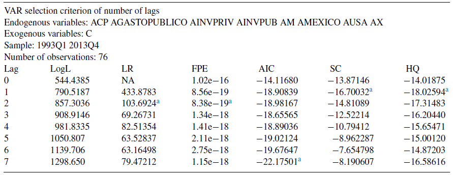
a Indicates the lag order selected by the criterion.
LR, modified sequential LR statistical test (each test at 5% level); FPE, final prediction error; AIC, information criterion Akaike; SC, information criterion Schwarz; HQ, information criterion Hannan-Quinn.
We consider that in accordance with the LR (sequential modified LR) criteria and the FPE (Final prediction error) criteria, the number of delays utilized shall be 2. Once the aforementioned tests have been carried out, we estimate the following VAR (2) model utilizing ordinary minimum squares, where Φ 1 y Φ 2 are the matrices of the coefficients, C t constitutes the vector of the constants, and ε jt is the vector of the random errors or innovations.
 (13)
(13)
The estimated VAR (2) system has 81 observations for each of the equations, including 8 independent variables.
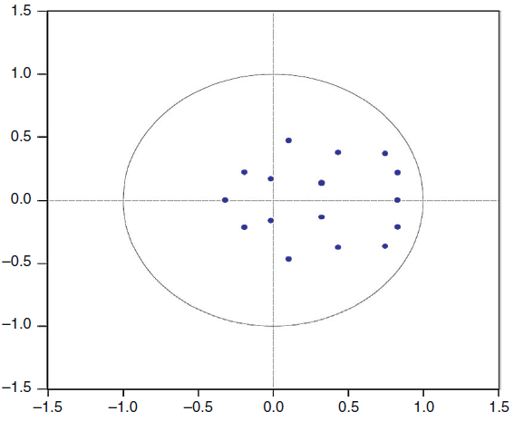
Stability test of the coefficients. In order to test the stability of the VAR system and its coefficients, the inverse roots of the characteristic polynomial of said matrix are required to not fall outside the circle. In this case, the results of the two stability tests that we carried out show that these fall inside the circle. For this we performed two tests, in the first we calculated the inverse roots of the polynomial, and according to the results the roots fall inside the circle; therefore, the estimated VAR meets the stability conditions as follows: the absolute value of the module decreases and tends toward zero (see Appendix Table 1), and then with the second test we supplement and confirm these results with a graphic analysis of the roots (Fig. 3).
Diagnostic tests for residuals (Table 9).. Subsequently we carried out a series of diagnostics on the Breusch-Godfrey autocorrelation tests on the residues. These are autocorrelation tests of the h order. According to the test, the null hypothesis of the absence of linear correlation was not rejected.
Table 9 Diagnostic tests for residuals.
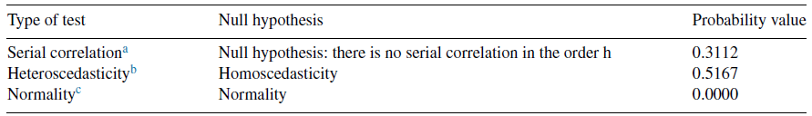
a Test of Breusch-Godfrey for the residuals from the first to the second order. The correlogram of the residuals is consistent with the absence of serial correlation until the twelfth lag.
b Test of Heteroscedasticity of for residuals with lags and without cross-terms.
c Normality test of Jarque-Bera.
According with the heteroscedasticity test the null hypothesis of the absence of heteroscedasticity was not rejected. And according with the normality test we found that the residues are not distributed normally.
Sensibility analysis. The following step consists on utilizing the technique developed by Pesaran and Shin (1998) to estimate a set of "generalized" response functions to the impulse (FGRI). The FGRI have the advantage of not depending on the order of the functions of the VAR model. These functions allow us to observe the "dynamic" response of a determinate variable in the face of shocks or unexpected changes in any other variable. Figure 4 shows how the cycle responds to the random shocks stemming from the variations in exports, public consumption, imports, and the GDP of the USA, respectively. As we can see, the FGRI were estimated in 40-quarter horizons and include 95% confidence intervals. For an impulse response function to be considered statistically significant, the confidence interval is required to exclude zero at some point within the 40-quarter horizon. In the first term, the stability of the system is observed, this shows the ability of the system to return to the stationary state. Figure 4 shows that the random shocks derived from innovations stemming from imports cause an expansion of the same, i.e., it has a pro-cyclical relationship, given that if imports increase so do the random shocks to the cycle, after 6 months the effect of the initial shock dilutes.
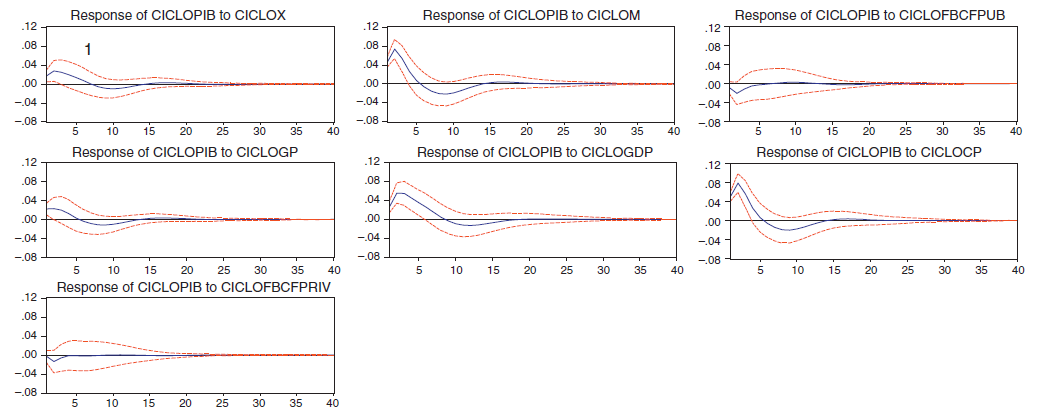
Likewise, the random shocks stemming from the variances of the American GDP induce an expansion of the Mexican cycle during the first 10 quarters, which dilutes after the 11th quarter. Imports also have a positive impact on the cycle, thus having a pro-cyclical effect. The expansion of exports and public spending generate a less pronounced positive expansion during the first 2 quarters. Lastly, it has been confirmed that investment does not influence the behavior of the cycle, and as such it can be confirmed that this variable is not adjusted to the balance of the goods market, as posed by the accelerator-multiplier model.
VAR Granger causality
Once we presented the results of the generalized functions of the VAR model, and the changes of the Mexican economic cycle before random shocks or innovations, we examined the Granger Causality relationship between the variables of the VAR model. Where X causes Y in the Granger sense if, and only if, the prognostic of Y is the result of the past values of X as well as the past values of Y. Granger (1969) distinguishes between unidirectional and bidirectional causality. There is a unidirectional causality of X-Y, if X causes Y but Y does not cause X. Now, in the case that none of the variables cause any of the others, it is said that the two series of time are statistically independent. In the case that the variables cause each other and there is a feedback relationship between them, it is said that there is a bidirectional causality between them. Once our eight variable VAR model has been estimated, as represented by Eq. (13), we carry out the Granger VAR/Block Exogeneity Wald causality test in order to examine the causal relationship between the 8 variables of the model; under this system, an endogenous variable can be treated as exogenous. We used the Wald statistics with a chi-square distribution in order to prove, in each equation of the model, the significance of each of the endogenous variables, as well as the significance of the combined endogenous variables delayed. The results are shown in Appendix Table 2. According to the value of the chi-square test statistics of 32.93 for the cycle of the GDP, it is shown that the 8 variables as a block cause a level of significance on the cycle of 0.0029, as per the Granger test. Where, only the American cycle individually causes the Mexican cycle.
Conclusions
The macroeconomic crises are linked to the cycles and emerge when the economy moves in an abrupt manner from a situation of expansion to one of contraction, thus seen at the peak of the cycle. (Marx, Hilferding, Schumpeter and Keynes)
In the analysis period we identified four economic cycles: the presence of three significant macroeconomic crises located at the peaks, where we can confirm a growing deceleration of the Mexican economy derived from the macroeconomic policies of public spending, which have been pro-cyclical.
All these variables had a pro-cyclical behavior, which was strange, especially due to the behavior of public spending (Public Consumption plus public investment); this is due to, above all, the stabilization policies and macroeconomic adjustment implemented since 1988.
The growing synchronization of the Mexican cycle with the American one, which explains the growing endogenization of the American crises by the Mexican economy, which is the result of the growing importance of imports and the American GDP on the Mexican economy. (Economic integration). That is in addition to the growing importance of the intra-industry commerce between both countries.
The USA crises, the dominant side of the relation, and the economic phenomena derived from them, with all their peculiarities of temporal, technical and organizational development, influence in a more resounding manner on the Mexican economy beginning from 2001.
According with the simulations of the stationary VAR (2) model, the dynamic of the cycles is primordially explained by: imports, the expansions of which cause a positive reaction of the cycle, shocks stemming from the GDP (external variables), and shocks stemming from private consumption (domestic variable); to a lesser extend exports and public consumption have influenced on the cycle. It is worth noting that the shocks stemming from private investment do not influence on the dynamic of the cycle, which explains the growing deceleration of the economy on the period. Other than that, all the variables have a pro-cyclical behavior and the dynamic of the cycle is associated with a macroeconomic pattern characteristic of a small rent-based open economy (private consumption, imports, and American GDP). In a developing country as is the case of Mexico, the expansion of investment is determined by the expansion of imports, here lies the importance of imports in the economic cycle. However, we observe that in the case of Mexico, private investment does not individually cause the cycle.
As a whole, the variables of the system caused, in Granger's sense, the cycle of the Mexican economy; and in particular was caused by the cycle of the United States of America, in Granger's sense.
REFERENCES
Brito, R. D. y Brianne, B. (2010). Inflation targeting in emerging economies: Panel evidence. Journal of Development Economics, Elsevier, 91(2), 198-210. [ Links ]
Calderón, C., Caire, G. y Sánchez, A. (2012). La estabilización macroeconómica mexicana de 1988-1992, una experiencia heterodoxa. En C. Calderón y V. M. Cuevas (Eds.), Macroeconomía abierta en América Latina: teoría y evidencia. México: EON. [ Links ]
Calderón, C. y Caire, G. (2012). Génesis y desarrollo de la crisis macroeconómica de 1995. En C. Calderón y V. M. Cuevas (Eds.), Macroeconomía abierta en América Latina: teoría y evidencia. México: EON . [ Links ]
Carare, A. y Stone, M. R. (2003). Inflation Targeting Regimes, IMF Working Papers 03/9. International Monetary Fund. [ Links ]
Granger, C. W. J. (1969). Investigating causal relations by econometric models and cross-spectral methods. Econometrica, 37(3), 424-438. http://tyigit.bilkent.edu.tr/metrics2/read/Investigating%20%20Causal%20Relations%20by%20Econometric%20Models%20and%20Cross-Spectral%20Methods.pdf. [ Links ]
Harrod, R. F. (1948). Towards a Dynamic Economics. London: Mac Millan. [ Links ]
Hilferding, R. (1971). El capital financiero. Cuba: Editorial de Ciencias Sociales, Instituto Cubano del Libro. [ Links ]
Juglar, C. (1889). Des crises commerciales et leur retour périodique en France, en Angleterre et aux États-Unis (2ème édition). Paris: Guillaumin. [ Links ]
Kalecki, M. (1935). A macrodynamic theory of business cycles. Econometrica, 3(3). https://archive.org/details/Kalecki1935.AMacrodynamicTheoryOfBusinessCycles. [ Links ]
Keynes, J. M. (2005). Théorie générale de lémploi, de l'intérêt et de la monnaie. Paris: Éditions Payot & Rivage. [ Links ]
Marx, K. (1965). Œuvres économie ly II. Paris: Éditions Gallimard. [ Links ]
Pesaran, M. y Shin, Y. (1998). Generalized Impulse Response Analysis in Linear Multivariate Models. Economics Letters, 58, 17-29. [ Links ]
Samuelson, P. A. (1938). Interactions between the multiplier analysis and the principle of acceleration. Review of Economics Statistics, (21). [ Links ]
Schumpeter, J. (1935). Théorie de lévolution économique. Paris: Librairie Dalloz. [ Links ]
1"the cycles always end in a general crisis, the end of a cycle and the beginning of another" Marx (1965) p.1149-1150.
2So that the "modern industrial cycles arise with capitalism and its expansion: expansion of the industry, expansion of external commerce over internal commerce, expansion of the universal market that successively attaches broad territories of the new world, Asia, Australia, Africa". Marx (1965), p.1149-1150.
3M kt' > D kt', (k = 1,..., n individual capitalists and t=time), that have their origin in the no realization of the necessary goods and luxuries produced (M) in Sector II, where IIc (v + pv), as well as in the capital goods produce in the period.
4Overproduction of mercantile capital that is not dispatched during the normal course of the capitalist cycle M kt ’ = D kt '.
6That allowed for the massive affluence of the individual capitals toward specific economic sectors.
8The fundamental macroeconomic problem in the decades of the 70s, 80s and 90s was inflation, so the government has brought up different strategies to fight it since 1982, thus, an orthodox adjustment policy was implemented, which led to a contraction and cuts in public spending that went from 36 to 25% of the GDP. Between 1988 and 1994 a heterodox anti-inflationary program comprised by two components was implemented. These components were: an orthodox section of budgetary discipline and a heterodox section of coordinated politics that aimed for the coordination of income based on tripartite agreements (the syndicates, the entrepreneurs and the government). The policies applied were successful in reducing inflation significantly, from June 1993 inflation remained below 10%, but it has not been able to boost economic growth and development. To this day, the issue of sustained economic growth remains in the government's agenda.
9with low credibility and clarity levels, and a high flexibility to achieve other objectives such as the structural reforms (Carare & Stone, 2003).
10Mainly, the imports of productive consumables and the absence of an industrial policy, which provide productive abilities, inhibited the accelerated effect of the offer. Policies that foster industrial growth, that generate productive capabilities, and that contribute to the increase of the economic potential and economic growth are still necessary in developing countries.
11The Mexican economy is in a stagnant economic phase context and sub-employment balance, so there is a need to implement an active fiscal policy to reactivate it in the short-term and to avoid compromising growth.
12Mexico is the third export partner of the USA, our exports of finished goods and hydrocarbons are directed toward this economy, and there is a growing dependence in the imports stemming from the USA.
13We have another different model of the cycle, accelerator-multiplier type, different developed by Kalecki (1935) according to this author, investment depends on the gap between earnings and the value ofaccumulated capital in a closed economy. I t = aΠ * t+1 - bK t
Appendix A. Supplementary data
Supplementary data associated with this article can be found, in the online version, at doi:10.1016/j.cya.2016.01.006.
Received: January 05, 2015; Accepted: February 16, 2016
 Este es un artículo publicado en acceso abierto bajo una licencia Creative Commons
