Introduction

In emerging markets, such as Mexico and Chile, the problems that may have market liquidity in times of international financial crisis have not been analyzed in sufficient depth. Mexico and Chile are two relatively open emerging markets in Latin America. This paper analyzes the effects on the stochastic discount factor of changes in liquidity in times of an international financial crisis.

During times of crisis the problems associated with the systematic market liquidity become stronger, because liquidity is lost and then the less liquid assets have higher prices. Systematic market liquidity refers to costs and time required to transform many of the assets into cash or vice versa. Systemic market liquidity decreases strongly in times of a crisis (e.g. Asia, 1997, Long Term Capital Management (LCTM) 1998 and Subprime, 2008), because there are fewer buyers willing to buy certain assets that we call illiquid. Therefore those assets have lower prices and higher required rates of return, Stambaugh (2003) and ^{Gibson and Mougeot (2004)}. Liquidity problems may refer to two situations: (1) there are not enough buyers of the good; or (2) that buyers who are in the market would buy only with a high discount (^{Diderich, 2009, p. 94}). Another way to observe that problem of liquidity in the market is that bid and ask prices separate (^{Diderich, 2009, p. 201}).

This work is divided as follows. This section is an introduction. Section 2 discusses the theoretical framework. Section 3 introduces the formal model. Section 4 discusses methodological issues. Section 5 discusses the analysis and results. Finally, the conclusions and recommendations section follows.

The model

The consumer-portfolio model, initially formulated by ^{Samuelson (1969)} and ^{Merton (1969)}, is amply discussed in the literature with slightly different variations. In the problem, a consumer can trade freely in assets i and maximizes the expected value of a discounted time-separable utility function, as in ^{Campbell, Lo, and MacKinlay (1997, p. 293)},

(3.1)

where δ measures the personal time preference, Ct+j is the investor's consumption in period i + j, and UCt+j is the period utility of consumption at t + j. Wealth Wt at t, as in ^{Pennachi (2008, p. 106)}, satisfies the following relation

(3.2)

where Wi,t is the proportion invested in risky asset i of the total wealth in period t , Ri,t is the return of risky asset i in period t, Rf,t is the return of the risk free asset in period t and yt is exogenous income wealth that the individual receives at period t. Notice that in this formulation, if the rate of return is zero, the return is one, which indicates that wealth is inter-temporally conserved.

The optimal consumption and portfolio plan must satisfy that the marginal utility of consumption today is equal to the expected marginal utility benefit from investing one monetary unit in asset i at time t, selling it at time t + 1 for Ri,t+1 and consuming the proceeds,

(3.3)

where Ψt is the information available to the individual at time t, a subset of the information available at time t, At. Dividing both sides in (3.3) by U'Ct, we get

(3.4)

where the stochastic discount factor mt+1 is equal to the stochastic inter-temporal rate of substitution δU'Ct+1/ U'Ct.

Note that if the returns of the n risky assets in the economy are the vector Rt, and 1- is a vector of ones, relationship (3.4) can be written as

(3.5)

where Rt has an unconditional non-singular variance-covariance matrix Σ.

An implication of this model and other inter-temporal asset pricing ones is that

(3.6)

where the return on one period riskless bond isRtf=1/ Emt+1|At and Rtf ∈ Ψt.

Estimation of Euler equation of consumption

In equilibrium, the conditional moment condition that the stochastic discount factor mt must satisfy conditional on previous information Ψt-1 is that the expected product of any return Rt with the discount factor must be equal to one,

(3.7)

According to ^{Hansen and Singleton (1982)} the discrete-time models of the optimization behavior of economic agents often lead to first-order conditions of the form:

(3.8)

where xt is a vector of variable observed by agents at time t and b0 is a p dimensional parameter vector to be estimated. Therefore:

(3.9)

Let us construct an objective function that depends only on the available information of the agents and unknown parameters b. Let g0b=Efxt;zt;b0. According to ^{Hansen and Singleton (1982)}, if the model in (3.9) is true then the method of moment estimator of the function g is:

(3.10)

The value of gTb at b=b0 should be close to zero for large values of T. In this paper, we follow ^{Hansen and Singleton (1982)} and choose b to minimize the function Jt

(3.11)

where WT is a symmetric, positive definite weighting matrix WT can be estimated minimizing

(3.12)

The choice of weighting matrix WT is such that it makes gT close to zero, taking into account possible heteroscedasticity and autocorrelation (HAC) behavior.

There are two advantages of estimating non-linear Euler equation under Generalized Method of Moments (GMM) as given in ^{Hansen and Singleton (1982)}:

1. The instrument vector does not need to be economically exogenous. The only requirement is that this vector be predetermined in the period when the agent forms his expectations. Both past and present values of the variables in the model can be used as instruments. Model estimator is consistent even when the instruments are not exogenous or when the disturbances are serially correlated.

2. Unlike the maximum likelihood (ML) estimator, the GMM estimator does not require the specification of the joint distribution of the observed variables.

To compute WT a consistent estimator of b0 is needed. This can be obtained by initially using Wt= Ir×r (identity matrix) and suboptimal choice of b in minimizing Jtb in (3.11), we get the values of bT. By using this value of b in (3.12) we get WT. Again by using the new values of WT,bT can be obtained by minimizing Eq. (3.11). We repeat this process until the estimates converge. According to ^{Hansen, Heaton et al. (1996)} this iterative GMM process is more efficient in small sample than a simple standard two-step procedure given by ^{Hansen and Singleton (1982)}.

Methodology

In this study, we analyze the performance of the Mexican and Chilean Stock Markets. For each asset, arithmetic returns were estimated. In each market, we consider a market index as benchmark. The market index used in the Mexican Market was the Total Return Index "Índice de Rendimiento Total (IRT)" and for the Chilean Market, the Santiago Stock Exchange Index "Índice de la Bolsa de Santiago (IPSA)," both indexes adjusted inclusive for cash dividends. The annual arithmetic rate of return and standard deviations of these indexes in the period of study are shown in Table 1.¹

Table 1 Mean and standard deviation of the daily market rate of return in Mexico and Chile. 

Daily rate of return.

Source: Own elaboration.

Table 1 shows the mean and standard deviation of the rate of returns during the whole period of study and each of the analyzed years. In 2008, there are negative rate of returns measured by IPSA and IRT. The same happened in 2011, when the prospects of the Mexican and Chilean economies weakened. The recovery was stronger during 2009 and 2010. The growth in 2012 was small, compared with those of 2009 and 2010. Volatility increased in 2008, then it decreased in the following two years, it increased again in 2011, and it has a slowdown in 2012, in both the IRT and the IPSA.

In each market, two equations were estimated using method of moments. If Eq. (3.8) is estimated for each return and the return for the risk free rate is subtracted for each of the returns, the following moment conditions must be satisfied:

(4.1)

where Ri,te is the excess return of asset i. The risk free rate used for Chile is the one day Chilean Interbank Rate, published by the Central Bank of Chile and, for Mexico, it is the 28 days Mexican Interbank Equilibrium Interest Rate (TIIE for its Spanish initials, Tasa de Interés Interbancaria de Equilibrio), published by the Bank of Mexico. If the CAPM is satisfied, mt can be written as a+bRi,te, see, for example, ^{Cochrane (2005, p. 152)}:

(4.2)

The excess market return is instrumented with the first three lags of the same variable, which are statistically significant in a Garch model.

Liquidity refers to the time and the costs associated with the transformation of a position in an asset into cash and vice versa. The CAPM, as many asset pricing models, assumes that the cost and time required for transforming financial wealth into cash are zero. Actually, the transformation of a position in some financial assets into cash can be expensive, particularly, if the asset has a low frequency of trading. The liquidity can refer to a particular asset or fund or to the entire financial market (i.e. systematic liquidity). An asset with low liquidity will command a different return from an asset with higher liquidity to compensate for the lack of liquidity. Similarly, if the asset return covaries with systematic liquidity, it would yield a liquidity risk premium to compensate for an event in which the asset differs in price along with the ability to liquidate it. This conjecture is consistent with the evidence that systematic liquidity is priced in equity markets, see ^{Pastor and Stambaugh (2003)} and ^{Gibson and Mougeot (2004)}.

^{Getmansky et al. (2004)} and ^{Aragon (2007)} analyze individual asset liquidity. These authors focus primarily on illiquidity as a cost factor that induces serial correlation in individual hedge fund returns and it may also provide an explanation for their higher expected returns. ^{Sadka (2010)} and ^{Brandon and Wang (2013)} study whether systematic liquidity risk is priced or not in the cross section of hedge fund expected returns. In ^{Sadka (2010)}, a high-liquidity risk exposure hedge fund portfolio (top decile) has a statistically significant percent higher annual return, on average, than a low-liquidity risk exposure hedge fund portfolio (bottom decile) during 1994-2008.

Liquidity effects on returns can be considered using directly liquidity-risky proxy measures such as in ^{Pastor and Stambaugh (2003)} or ^{Amihud (2002)}. This article follows an alternative approach, which considers the effect of liquidity on excess return measures (i.e. alphas and appraisal ratios), as in ^{Agarwal and Naik (2004)} and ^{Getmansky et al. (2004)}. Each year, each stock in the market is classified as high liquidity stock or low liquidity one depending if the stock traded more than 200 days in the year or less. The effect of liquidity was considered in two ways: the effect on the constant or on the beta of the stochastic discount factor. The effect is statistically measured using a Chow test. The variable I has a value of one if the stock has more than 200 quotes in the year and zero otherwise. The moment conditions become

(4.3)

Analysis and discussion

If liquidity does not affect the stochastic discount factor, the coefficient of ag and bg in Eq. (4.3) must be equal to zero. For Mexico, in the two step estimation, ag or bg, or both are statistically different from zero in all years in the period 2007-2009, see Table 2. Using the GMM estimation, either of the coefficients ag or bg is different from cero in the period 2007-2009 and the year 2012, see Table 3. There is a liquidity effect in the stochastic discount factor in Mexico in the period 2007-2009, the period of the international financial crisis and the year after. The same effects are confirmed with the Chow Test, which shows that there is liquidity effect in the stochastic discount factor in the period 2007-2009 using the two step estimation and the iterated GMM estimation, see Table 4. In the iterated GMM estimation, there is an effect in the year 2012, but it is weak: the probability of that either coefficient is equal to zero is 5.2%.

Table 2 Coefficients for Mexico with the IRT Index, GMM with two steps. 

Coefficients a0, a1 from assets with more than 40 quotes in a year, ag, bg with more than 200 quotes in a year.

*Statistically significant at 90 percent level.

**Statistically significant at 95 percent level.

***Statistically significant at 99 percent level.

z are HAC standard errors.

Source: Own elaboration.

Table 3 Coefficients for Mexico with the IRT Index, iterated GMM. 

Coefficients a0, a1 from assets with more than 40 quotes in a year, ag, bg with more than 200 quotes in a year.

*Statistically significant at 90 percent level.

**Statistically significant at 95 percent level.

***Statistically significant at 99 percent level.

z are HAC standard errors.

Source: Own elaboration.

Table 4 Chow Test for Mexico. 

Joint hypothesis: Constant and slope coefficients of stocks with more than 200 quotes per year is zero.

Source: Own elaboration.

For Chile, the effect of liquidity in the period 2007-2009 is also observed, the period of the credit financial crisis and the year after. This effect is observed using the two stage estimator and the iterated GMM estimator, see Tables 5 and ⁶. In addition, in 2011, the two stage estimator and the iterated GMM estimator show that there is a liquidity premium effect, see Tables 5 and ⁶. These effects are confirmed using a Chow Test for the market liquidity premium that shows that there is at least one coefficient related to the liquidity premium that it is statistically different for zero in the years in the period 2007-2009 and 2011, see Table 7, for either the two stage estimator or the iterated GMM estimator, that is, in the period of the credit financial crises, the year after and in the year 2011. Iterated GMM estimation has better small sample properties than two step estimation (^{Hansen et al., 1996}). However, large sample statistical properties of both estimators are roughly similar.

Table 5 Coefficients for Chile with the IPSA Index, GMM with two steps. 

Coefficients a0, a1 from assets with more than 40 quotes in a year, ag, bg with more than 200 quotes in a year.

*Statistically significant at 90 percent level.

**Statistically significant at 95 percent level.

***Statistically significant at 99 percent level.

z are HAC standard errors.

Source: Own elaboration.

Table 6 Coefficients for Chile with the IPSA Index, iterated GMM. 

Coefficients a0, a1 from assets with more than 40 quotes in a year, ag, bg with more than 200 quotes in a year.

*Statistically significant at 90 percent level.

**Statistically significant at 95 percent level.

***Statistically significant at 99 percent level.

z are HAC standard errors.

Source: Own elaboration.

Table 7 Chow Test for Chile. 

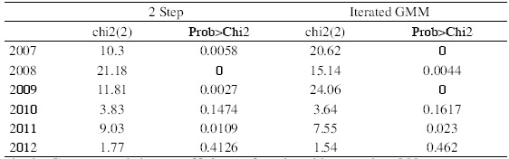
Joint hypothesis: Constant and slope coefficients of stocks with more than 200 quotes per year is zero.

Source: Own elaboration.

In the model, the liquidity effect in the stochastic discount factor can be a constant or depend on the level of an index. For Mexico, using the two steps procedure, there is a statistically positive constant liquidity effect in 2008 at the 95 percent significant level, see Table 2. The effect is more noticeable using the iterated GMM, see Table 3. The 2008 effect becomes statistically significant at the 99 percent level. In addition, a statistically positive constant effect is observed in 2007 at the 95 percent of significance level.

For Chile, using the two stage procedure, there is a constant positive liquidity effect in the year 2007 at the 95 percent significance level and in the year 2008 at the 99 percent significance level, see Table 5. Using the iterated GMM, the constant positive liquidity effect is observed in all years in the period 2007-2011, but it is statistically significant at the 99 percent level in 2007 and 2009, and at the 95 percent level in the years 2008 and 2011, see Table 6.

The sensibility of the stochastic discount factor to the index to liquidity can differ with the level of the index. A positive (negative) sign of b_g implies that more liquid stocks are less (more) discounted than more (less) liquid stock the higher the index. For Mexico, the sensibility to the IRT index show statistically significant differences with liquidity. The stochastic discount factor using the IRT Index as market index shows a higher discount for the more liquid assets in the years 2007 and 2009 in both the two step and the iterated GMM procedures. It is noticeable that the sensibility is not statistically significant in 2008, a year when the effects of the global liquidity crisis were stronger in the region. It is also a year in which the IRT Index has an average rate of return negative, see Table 1.

For Chile, the excess sensibility of the stochastic discount to the index to liquidity is statistically negative in 2009 and positive in 2008 and 2011 with the two step method, see Table 6. Using the iterated GMM methods, the excess is positive for the years 2007 and 2008 and negative for the year 2009, see Table 7. Notice that in 2008, a year in which the average IPSA return rate was negative, the stochastic discount shows a greater sensibility to the index for the more liquid assets with a statistical significance of 99 percent. This result is observed with the IPSA Index as a market index and using the two step and the iterated GMM methods, see Tables 6 and 7.

Conclusions

The stochastic discount factor can provide evidence of mispricing of assets, even though literature frequently discusses these issues using asset pricing models such as the CAPM or multifactor models. There is a liquidity premium factor in the Mexican and Chilean economies in some years of the period of study, 2006-2012. The GMM method can give different inferences if a two stage estimator or an iterated one is considered. However both methods offer statistical evidence that there is a liquidity premium factor in the years of the International Credit Financial Crisis, 2007-2008 and the year after for Mexico and Chile, except in 2007 for Chile with the two step procedure.

The liquidity effect can be constant or it may depend on the level of an index. A statistically significant constant effect is observed using the iterated GMM for Mexico in the years 2007 and 2008, and for Chile, in the years 2007-2009 and 2011.

In Mexico, the sensibility of the stochastic discount factor to the IRT as market index is statistically smaller if the stocks are more liquid in the years 2007 and 2009 using the iterated GMM. For Chile, the sensibility of the stochastic discount factor to the IRT as market index is statistically smaller if the stocks are more liquid in the years 2007-2009 using the iterated GMM.

The results warrant a careful interpretation considering a possible model misspecification, which can result from missing factors, a non-linear factor model, inadequate instruments or over-identification issues, which are left for further extensions.