Introduction

The Microfinance Institutions (MFIs) started their operations in Bangladesh and India at the beginning of the 70's with the idea of giving small short-term credits (less than 100 USD and until one year) to the poorest people without asking for collateral. In order to get the loan repaid, local reputation and group borrowing were used as a social pressure, for more details see (Consultative Group for Assistance to the Poorest, ^{CGAP, 1996}, and ^{Roodman and Qureshi, 2006}).

The Microfi model used in Bangladesh and India was so successful¹ that it was imported to Latin America in the late 80's; mainly to Peru, Bolivia and Mexico. Originally, it was intended to diminish poverty and favor the social inclusion of the poorest; see, for instance, ^{Armendaris and Morduch (2011)}, ^{Olivares-Polanco (2005)}, and ^{Weiss and Montgomery (2005)}. However, the capital donors were exhausted and competition changed the incentives of the lending process, so the MFIs faced the need of changing part of their lending methodologies by raising interest rates or going to new donors' rounds on a global financially constrained scenario; see, for instance, ^{Morduch (1999)}, ^{Cull el at. (2010)}, and ^{Serrano-Cinca y Gutiérrez-Nieto (2014)}.

After the subprime crisis, there was scarcity of new donors, so the financial health of MFIs became a concern to keep them working. Thus, the market discipline began to apply to these partially new institutions devoted to diminish poverty. As a result of this changing environment, many of them went to bankruptcy or got into financial stress; a deeper insight on this process can be found in ^{Servin et al. (2012)}, ^{Hermes et al. (2011)} and ^{Karim (2011)}.

Mexico was not isolated to these new micro-financial activities, the first Mexican Microfinance Institutions started their operations in the late 90's in Oaxaca and Chiapas as non-profit institutions, reaching their highest number on 2011, 67 MFIs, as reported by the Microfinance Information Exchange (MFIX). At the end of 2013, after a big restructure on the industry, the number of reported MFIs by the MFIX was 52 institutions operating in México with a total gross loan portfolio of USD 2.6 billion and almost 6 million of active borrowers as shown in Figure 1.

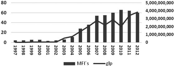
Source: Author's own elaboration with data from the Microfinance Information Exchange (MIX Market).

Fig. 1 Number of IMFs and their portfolio (USD dollars) in Mexico 1997-2012. Annual frequency. 

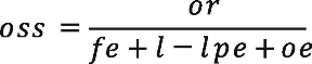
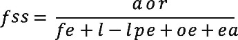
The effects of the subprime crisis radically changed the MFIs scenario, exhausting the chance of a new round of donor's money, they need to create their resources. Therefore, the main problem for the MFIs operation was to expand the number of attended clients without losing financial sustainability. Using the criteria defined by the Consultative Group for Assistance to the Poorest (CGAP), the financial sustainability of a MFI is given by two leading indicators (oss and fss ); see, for instance, (^{Christen et al. (1995)}, ^{Rosenberg et al. (2003)}, and ^{Bogan (2012)}).

These measures are defined by the two following equations:

(1)

(2)

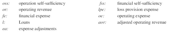
variables are defined as follows:

Although there are several studies analyzing the way in which the subprime financial crisis affected the MFIs in the long-run behavior, some of them considered the microcredit industry as a whole. In the best scenario, some investigations have considered differences on the geographic location of the MFIs.² However, it is missing a study among their sizes, margins, and costs, and this paper will be concerned with this respect.

There are some other studies attempting to capture the effects of the relation and competition among the MFIs. ^{Louis and Baesens (2013)}, ^{Mersland and Strøm (2010)}, and ^{Hermes and Lensink (2011)} consider the evolution of these organizations (time series effect) and competition between them (cross section effect "between efect"). Also, there are some efforts in measuring the impact of the MFIs against poverty, see, for instance, ^{McIntosh et al. (2011)} and ^{Imai and Azam (2012)}.

We will be mainly focused on the MFIs risk management in Mexico taking into account their heterogeneity and industrial relations from 2007 to 2012.³ Our hypothesis is that the MFIs sector has become a competed industry between 2007 and 2012. Not only because the scarcity of new donors, but also for the existence of many organizations that erode the margins of the firsts MFIs increasing the interest rate in all the industry. This gives to the clients the possibility of defaulting without losing all their access to credit due to competition. These circumstances increase the operational cost in the sector, but this phenomenon is asymmetric along the sample, being worse for the small organizations.

We will be using, in what follows, two quantile regression methods, specifically the quantile regression proposed by ^{Koenker and Bassett (1978)}, and the non-separable disturbance technique for panel data suggested by ^{Powell (2013)}. We use these techniques because they have the capacity of analyzing the heterogeneity in size, costs, and income in the Micro Finance Institutions industry without making any distribution assumption of the quantile regression, and maintaining the ability of capturing the competition effect within the industry given by the panel data methodology.⁴

It is also important to point out that ^{Crabb and Keller (2006)} analyzed risk factors in a sample of different countries by considering as a risk measure (Portfolio at Risk>30 days), loan sizes, GDP by country, gender, etc. However, the period of study is before of the subprime crisis. The main contribution of this paper is to analyze for the Mexican case during the world crises by using quantile methodologies.

In section 2, we perform a descriptive analysis of the variables and panel unit roots tests, specifically the test are from ^{Breitung and Meyer (1994)} and ^{Levin et al. (2002)}. We will be using the pooled regression, with fixed and random effects, for traditional panel data and compare them. We obtain that the pooled regression is the best model for the traditional panel approach. In section 3, we present the quantile regression method (^{Koenker and Bassett, 1978}) and a regression for a fixed effect panel with non-separable disturbance as proposed by ^{Powell (2013)}. Finally, we provide conclusions and acknowledge limitations.

A panel data approach

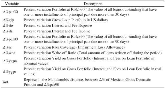
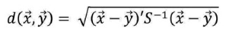
As we stated previously, we attempt to explain the change in the risk exposure (percent variation of the Portfolio at Risk greater than 30 days) of the MFIs, denoted as par30 , as function of the change of their business size (percent variation of their Gross Loan Portfolio in US dollars), glp , the change on their financial costs (percent variation of their Interest and Fee Expense), ife , the change on their financial revenue (percent variation of their Interest and Fee Income), ifi , the change on their non-performing loans (percent variation of their Portfolio at Risk>90 days), par90 , the change on their financial strength (percent variation of their Risk Coverage), rc , the change on their operational efficiency (percent variation of their Write off Ratio), wor , the change on their nominal and real margins (percent variation on their Yield on Nominal and Real Gross Portfolio), ygpn and ygpr , respectively (see Appendix A). Finally, md , stands for the Mahalanobis distance between the percentage change of Mexican gross domestic product and the percentage change of par 90 in order to capture the effect of economic environment over the risk factors (see Appendix B).

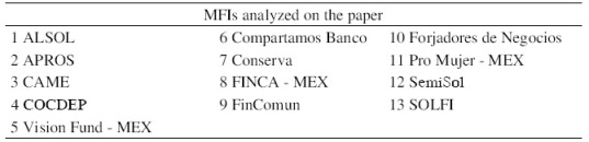
We use data of 13 Mexicans MFIs⁵ provided by Micro Finance Information Exchange (MIX) from 2007 to 2012⁶ (see Appendix C). We have one yearly observation for each variable on every MFI. This means a balanced panel that avoids the survival bias or a self-selection bias by constraining the study to the financially healthy and transparent organizations during the studied period. It is important to point out that our results hold only for financially healthy organizations that have the incentive of making public their information voluntarily for attracting potential investors with a lower cost. If we extend the study to other MFIs that are not publishing their complete data in the studied period, heterogeneity will still be greater distorting the results.

Descriptive analysis and unit roots panel data test

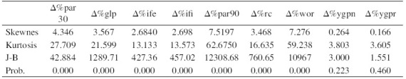
In this section, we first show that there is non-normal heterogeneity on the panel. For doing so, we made some descriptive statistics on the aggregated panel variables (over the MFIs). As an important result, showed on the Table 1, is the absence of normality on all variables, except the yield on nominal and real gross portfolio, ygpn and ygpr , respectively. The normality assumption was examined by using the ^{Jarque and Bera (1987)} test, which is based on the sample skewness and kurtosis. Although this test may present some problems on small samples, the values of the skewness and kurtosis eliminate some doubts about the result of the test.

Table 1 Descriptive Statistics of the Variables in the Model. 

Source: Author's own computation with Microfinance Information Exchange MIX, and Stata 12.1.

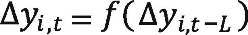
After presenting the normality test for the studied variables, we perform the panel unit root tests. For the sake of clarity, we present a brief review on them and comment the implications of the sample heterogeneity over the test results. Both panel unit root test, provided by ^{Levin et al. (2002)} and ^{Breitung and Meyer (1994)}, begin with the calculation of the panel errors, ¿_it, as those generated by the regression of the changes on the contemporary panel realizations, Δy _{i, t} , as function of the lagged changes on the variables, Δy _{i, t− L} , which can be stated as:

(3)

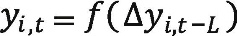
The second set of panel errors, v̂_it, given as a result of the panel regression on the contemporary panel realizations,y _{i, t} , as function of the lagged changes on the variables Δy _{i, t− L} , can be written as follows:

(4)

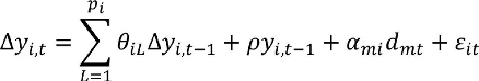
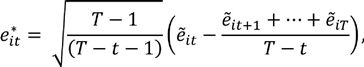
where the lag order is independent for each variable i , and, L= 1,...,p _i . This methodology can be viewed as the panel extension of an ADF test. For this reason, we can expect a low power test if we depart for the normality assumption. This low power is caused by the kurtosis excess because the rejection area is bigger than the assumed. By using the sample standard deviation σ̂_εi, given by the panel unit root test specification in equation (3), we have the following expression:

(5)

Here, the intercept,ρy _{i, t−1} and the trend, α _mid_mt depend on the specification. The standardized errors ẽ _it and ṽit, for both panel specifications, are constructed as and It is important to emphasize the normality assumption over the errors ε_it over which both tests are based. In the specific case of the ^{Breitung and Meyer's (1994)} test, the lagged panel errors are defined as the difference between the actual standardized lagged panel errors and the average of their standardized lagged past realizations, corrected by the sample size, i .e ., a forward orthogonalization:

(6)

The second part of the test is to define the test statistic as function of the standardized panel errors, given in equation (4).

As usual the intercept, ṽ_i1, and the trend , are optional, that is:

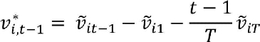(7)

Hence, a pooled regression is performed between the lagged panel errors, given in (6), and the test specification given as function of the standardized panel errors in equation (7). This is expressed as

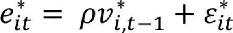(8)

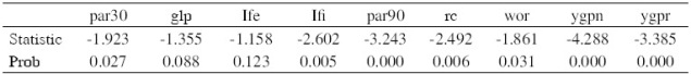
In this case, the null and hypothesis for the ^{Breitung and Meyer's (1994)} test is a stationary panel, H ₀: ρ=0. In Table 2, we show the t -statistics probabilities of the performed panel unit root test.

Table 2 Breitung and Mayer Unit Root Test. 

Source: Author's own computation using Microfinance Information Exchange (MIX), and Stata 12.1.

The test from ^{Breitung and Meyer (1994)} is performed just like a "panel corrected" ADF test. Therefore, it shares the low power characteristic. We can see that the business size (percent variation of their Gross Loan Portfolio in US dollars), glp , and the change on their financial costs (percent variation of their Interest and Fee Expense), ife , have unit roots at the 5% confidence interval. While the risk exposure (percent variation of the Portfolio at Risk greater than 30 days), par30 , and the change on their operational efficiency (percent variation of their Write off Ratio), wor , present unit roots at a 1% level of significance.

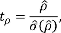
If we consider the effect of the kurtosis excess on the sample, we note that the rejection region is longer than the one proposed under the normality assumption. Thus, there may be false negatives (false H ₀ rejections). To amend this, we use the test provided by ^{Levin et al. (2002)}, whose null hypothesis is a non-stationary panel H ₀: t_ρ=0. The statistic from ^{Levin et al. (2002)} is constructed using the idea of a t -test on a partitioned regression estimator (Frisch-Waugh Theorem) for the unit root, which leads to:

(9)

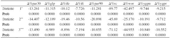
where the unit root parameter, p̂, is given as the regression parameter between the standardized lagged changes in panel errors ẽ_i,t, stated in (3), and the standardized panel errors in equation (4). That is, 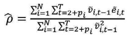. The standard deviation is given by , where . Under this framework, the test assumes that each one of the time series is explosive (has unit root); however, the test is using the normality assumption. The results of the test are shown in Table 3.

Table 3 Unit Root Levin Lin Chu Test. 

1* none, 2* intercept, 3*** intercept and trend.

Source: Author's own computation using Microfinance Information Exchange (MIX), and Stata 12.1.

The most remarkable result showed in the table (3) is that none of the series presents an explosive behavior (unit root), this result allows us to make the panel analysis presented in the next section emphasizing the effects of heterogeneity in the panel data analysis. We compare our results with those obtained using the traditional panel approach based on the normality assumption of the errors and average behavior of the sample. For doing that, we propose the pooled regression analysis (10), fixed effects panel analysis in (11), and random effects panel model in (12).

(10)

(11)

(12)

Although the three model specifications are very similar, they present great differences. In the case of the pooled regression (10), there is just one common intercept for all the MFIs. That is, there are not specific differences among them and that their behavior along the time is practically the same. Thus, for the sake of simplicity the best model is the one with fewer parameters (the pooled model with the common intercept β0 and the slope vector βi). It is important to point out the that ordinary least squares provide consistent and efficient estimates.

In the second case, the fixed effects model (11), there are specific idiosyncratic effects that are correlated with each of the MFIs. Hence, the least squares estimator is biased due an omitted variable problem. The problem is solved by adding an intercept for each of the IMFs losing generality in the analysis. This means that the sample parameters cannot be extrapolated to the entire population. In this case, the fixed effects model can be stated in a compact form as:

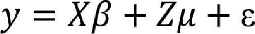(13)

The term of error is discomposed in two parts ε=Zμμ+v, and its vector of parameters is calculated by means of:

(14)

where ε̃ = ȳ.. - β̃ x̄.., Zμ = IN⊗lT, P = Zμ (Zμ'Zμ)−1Zμ', and Q=INT − P IN. It is important to remember that IN and INT are diagonal matrices of order N and NT, respectively, and lT is a vector of 1's of order T.⁷

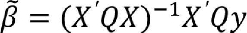
While in the third case, the random effects model, there is a group of specific random elements that are not distinguishable from the errors on the model but those random elements are uncorrelated with the regressors. In this case, the information obtained from the panel data sample can be extrapolated to the population. The random effects model assumes that μi∼IID(0,σ2μ) and vit∼IID(0,σ2v). The model also assumes that Xit is independent of μi and vit, respectively. In this case, the model parameters need to be obtained by Generalized Least Square (GLS) using:

(15)

where is a NTxNT matrix and with . It is important to point out that the unknown random effect is independent of the error term, thus the variance can be spread in two uncorrelated terms, and this means that σ² ₁=Tσ² _μ+σ² _v. Once we have explained the models briefly, we show in Table 4, the results for the three models specification (Pooled Regression, Fixed Effects, and Random Effects).

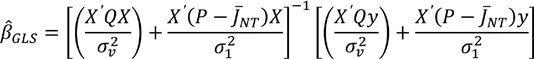
Table 4 Results of Pooled Regression, Fixed Effects, and Random Effects. 

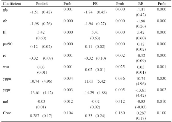
Source: Author's own computation using Microfinance Information Exchange (MIX), and Stata 12.1.

After analyzing the results in Table 4, we can see, in the fixed effects approach, that the md is not significative. For the pooled and random effects model specifications, it can be appreciated that all variables, except the intercept, are statistically significant at the 5% level. Moreover, the change in the Write off Ratio (the operational efficiency) is not significant only for the fixed effects model at the 1% level only.

The fact of having two models with all their variables statically significant at the 5% confidence interval (random and pooled) creates the need for choosing between the models. For our purpose, it is important to remember that we should compare these three models using ^{Hausman,'s (1978)} test to discriminate between the fixed and the random effects models. In this case, the null hypothesis is the existence of random effects due the orthogonality hypothesis between the common effects and the regressors. Hence, the estimated coefficients of the Generalized Least Squares (GLS) are consistent and efficient. For discriminating between the fixed effects model and the pooled regression, we may use the (^{Breusch and Pagan, 1979}) test where the null hypothesis is that the pooled regression is the correct specification and that the Ordinary Least Squares estimated parameters are consistent and efficient because there is not a missing variable problem.

In the case of the MFIs risk exposure, if we carried out just a traditional panel approach, we may choose the pooled model. ^{Hausman's (1978)} test indicates that the fixed effects model is preferred to the random effects model, but the (^{Breusch & Pagan, 1979}) test indicates that the pooled regression is preferred over the fixed effects model. We show these results on Table 5.

Table 5 Hausman and Breusch-Pagan test for the models in Table 2.4. 

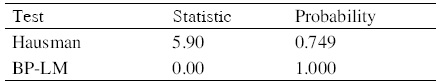
Source: Author's own computation using Microfinance Information Exchange (MIX), and Stata 12.1.

After the analysis of the MFIs credit risk exposure using the traditional panel approach, we may think that all micro credit institutions are controlling their risks in the same way since the best model is the pooled regression, but this conclusion does not explain the difference in size and financial success between them, neither the kurtosis excess in their operational and financial measures. In order to improve the analysis, we use the quantile regression approach. This will be carried out in the next section.

Quantile regression in panel data

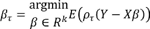
As explained previously, the quantile regression is applied to capture heterogeneity in the model without making any assumption on the sample distribution. It suffices that the sample distribution converges to the population distribution. The model was originally proposed by ^{Koenker (2004)} by solveing the optimization problem given by the following expression:

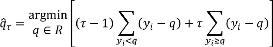(16)

After simplifying the above problem, we have to minimize the distance among the observation and its quantile . In this case, the conditional quantile regression is given by Q _{Y| X} (τ ) = Xβ _τ , 0 < τ < 1, which may be obtained for a particular distribution Y and parameters β _τ by solving:

(17)

With the intention of making both sections comparable, we take the same model as the used for the traditional panel approach. The quantile panel regression estimators are shown in Table 6.

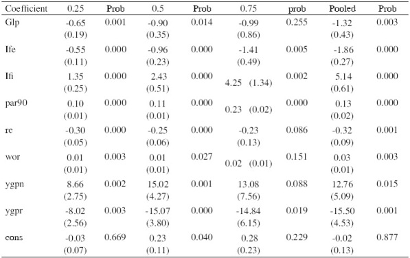
Table 6 Quantile Regression. 

Source: Author's own computation using Microfinance Information Exchange (MIX), and Stata 12.1.

In the results obtained in Table 6, we do not consider variable md , because is not significative at any level. The intercepts are not significant for any quartile at 5% confidence level. Also, we can see that the changes in the gross loan portfolio (size), glp , and the change in the write off ratio (operational efficiency), wor , are both not significant for the 0.5 quartile at the 1% significance level. In the same way, the change in the Gross Loan Portfolio (size), glp , the change on risk coverage (financial strength), rc , the change on the write off ratio (operational efficiency), wor , the change on yield on nominal gross portfolio (nominal margin), ygpn , and the intercept are not significant for the 0.75 quartile at 5%. The change in yield on real gross portfolio (real margin), ygpr , is not significant at 1% confidence level. Finally, the change on yield on nominal gross portfolio (nominal margin), ygpn , is not significant for the pooled sample.

These differenced results showed in the first quantile panel confirm that the heterogeneity of the data affects the regression results and that this heterogeneity arose mainly from the .75 quantile. It means that the risk exposure of an MFI located in the 0.25 quartile will behave differently from the risk exposure of other MFI located in the 0.75 quartile. As stated previously, the intercepts were not significant in this model for none of the quartiles. For this reason, we will be using the quantile regression model with non-additive fixed effects proposed by ^{Powell (2013)}. This model may be stated in the following way:

(18)

In this case, the parameter vector is obtained using the Generalized Method of Moments (GMM) estimation by assuming some instrumental variables of the form:

(19)

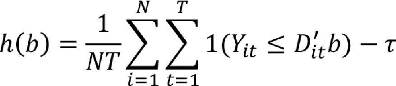
where the term U^* _it = f (α_i,U_it ). In this model, the structural quantile function (SQF) is given by:

(20)

This quantile function leads to a probability function P(Y_it ≤ D'_itβ(τ)|D_it) = τ. In Powell's model is possible that the probabilities can be different among cross section. In our case,τ _i can be different among the IMFs. Hence, the GMM representation is defined considering two Sample Moments as:

Sample Moment 1

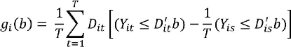(21)

Sample Moment 2

(22)

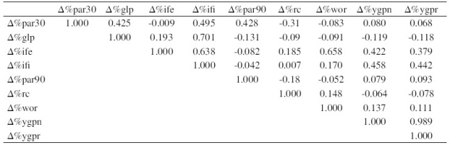
We can see that the last equation is similar to the cross-sectional quantile moment in taking τ _i instead of τ . The model only allows us to set one explanatory variable due to the use of instrumental variables for the years having a single independent variable. We show the non-additive fixed effects quantile panel model in Tables 7-⁹. The correlation matrix appears in Appendix C.

Table 7 Quantile Fixed Effect, Regression in Panel Data with Non-Additive Error Term Portfolio at Risk (par30) in function of the change in the gross loan portfolio (glp) and time. 

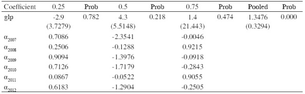
Source: Author's own computation using Microfinance Information Exchange (MIX), and Stata 12.1.

Table 8 Quantile Fixed Effect, Regression in Panel Data with Non-Additive Error Term Portfolio at Risk (par30) in function percent variation of portfolio at risk 90 (par90) and time. 

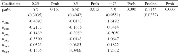
Source: Author's own computation using Microfinance Information Exchange (MIX), and Stata 12.1.

Table 9 Quantile Fixed Effect, Regression in Panel Data with Non-Additive Error Term Portfolio at Risk (par30) in function of interest and fee income (ifi) and time. 

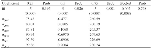
Source: Author's own computation using Microfinance Information Exchange (MIX), and Stata 12.1.

From the last three tables, the reader may see that only the portfolio at risk at 90 days (non-performing loans), par90 , and the interest and fee income (financial revenue), ifi , are significant. In the case of the portfolio at risk greater than 30 days (risk exposure), par30 , the quartiles are significant except the first (0.25). This is not a surprising result because the smaller firms with less exposed portfolio must accept almost every client in an attempt to grow. They cannot have a big revenue because they usually compete using their price. They also were the most affected on the crisis years. We emphasize in the change on the borrower quality expressed in the changes on the time parameters associated with par90 in Table 7. The above analysis shows the heterogeneity caused through time, that is, the business environment changed drastically in the sample and that the MFIs reacted in different ways to these changes depending on their risk exposure and size.

Conclusions

As we state at the beginning of this research, the Micro Finance industry became competed during the period of the sample (in the crisis years). Competition affected in different ways firms the industry. In the statistical descriptive analysis, it was shown that there exist differences among MFIs in a Jarque-Bera context; being the exception Δ%ygpn and Δ%ygpr . Moreover, it was examined whether there is an explosive behavior in the variables by using a unit roots test for panel data. By applying Breitung and Meyer test, we found that Δ%ife shows a non-normal behavior, which can be interpreted as the increase in the operation cost in different MFIs. As a consequence, some of them do not reach an economy of scale; however, under Levin-Lin-Chu test none of the variables show an explosive behavior.

In analyzing whether there exist any difference among the MFIs captured in a panel data approach, we found that the pooled model is the most appropriated under the normality assumption, implying that all the MFIs behaves in the same way and that their behavior is constant through time. Consequently, we may conclude that Δ%par30 as a function of the specified variables in model (8) is the most appropriated approach (^{Crabb and Keller, 2006}).

On the other hand, when we performed the quantile regression, we provide empirical evidence of differenced responses, through time and between quartiles, to changes in some credit risk factors. In the period of analysis 2007-2012, including the subprime crisis, we found that the 0.75 percentile of the IMFs sample is the source of a significant part of heterogeneity. Moreover, most of the regressors become statistically non-significant. As a result, we found, for 0.25, 0.50, and 0.75, that Δ%ife , Δ%ifi , Δ%par90 , and Δ%ygpr are significant. Consequently, the MFIs do not consider the size (glp ), risk hedging (rc ) and loses (wor ) for their risk management.

Finally, the quantile panel data approach proposed by ^{Powell (2013)}, with fixed effect in a non-additive form, obtains coefficients in a semi-parametric form by using a GMM (Generalized Method of Moments) for two moments. We found that only Δ% par90 and Δ%ifi are significant at the level of quantile at 0.50 and 0.75. In other words, the MFIs during the period 2007-2012 consider only for the risk management their semi-controlled risk (par90 ). In other words, the IMFs only consider for credit risk management the income they can attain.