


 text new page (beta)
 English (pdf)
 Article in xml format
 Article references
 Send this article by e-mail
 Cited by SciELO
  Similars in
SciELO
Similars in
SciELO 
 Permalink
Introduction
Pension savings in Mexico are among the most important private reserves in Mexico. The most used pension schemes in the country are the Defined Benefit (DB) and the Defined Contribution (DC) ones. The latter are also known in Mexico as SIEFOREs1 and represent the most important private reserve in the country by following a life cycle investment regime. At June 30, 2013, this pension funds managed MXN$ 2.8 trillions in savings. According to Albo et al. (2007), the amount of savings in SIEFOREs, as of 2050, will be 23% of Mexican GDP. For further reference about SIEFOREs, a more complete review of the pension fund system in Mexico is given by IMEF (2006).
According to the previous facts, to measure the portfolio management performance of these pension funds is a vital task to do in order to secure the sustainable growth of their wealth in the long-term. A natural solution to this issue is to develop a market-cap weighted benchmark of all the publicly traded SIEFOREs in Mexico but unfortunately this sort of benchmark carries several theoretical and practical issues that will be considered in detail next. In a first review of asset pricing models critiques, Roll (1977) observed that the real market portfolio is unknown and proves that the CAPM tests and critiques cannot hold because the market portfolio proxy could be mean-variance inefficient. Despite this fact, he recommended the use of market-cap benchmarks as market portfolio proxies.
As we will note in the literature review, there have been several critiques to the use of this sort of benchmark and various proposals have been made, such as the use of fundamental indexing (for equity markets) or the use of the Max Sharpe ratio portfolio, the equally weighted (1/N) or the minimum variance portfolios. Also, some other theoretical proposals use a linear combination of the last two aforementioned cases. By the fact that there is no public performance benchmark for each type of SIEFORE in Mexico and departing from the aforementioned weighting methods, the present paper makes a first proposal to this issue: To use a minimum variance portfolio as benchmark (henceforth min variance for simplicity in the reading) to measure the performance of the Investment Policy Statement (IPS) allowed by CONSAR2 (2012) and, as consequence, to measure the performance of all the SIEFOREs in Mexico (independently of their life cycle target).
One of the reasons that motivate this first proposal of using the min variance portfolio as benchmark is that this weighting method does not need any assumption about the expected returns vector and, therefore, is theoretically more flexible than other portfolios, such as the Max Sharpe one. This sort of weighting method is also more appropriate (also theoretically speaking) than other alternative or "naïve" schemes such as the 1/N or the fundamental indexing. By following this and by observing that the Max Sharpe portfolio is the theoretical geometrical spot of the real market portfolio,3 it is necessary to compare the performance of the min variance benchmark against a Max Sharpe portfolio. By following Amenc et al. (2012), it is also desirable to test the min variance portfolio against another weighting method such as the Max Sharpe one or a 50-50% linear combination portfolio between the min variance and the Max Sharpe, leading us to test the next general hypothesis in our paper: "The minimum variance benchmark of the SIEFOREs' IPS is as mean-variance efficient as the Max Sharpe one and the MV-Max Sharpe but preferable than these by its risk exposure and representativeness". If this hypothesis holds, then it will be preferable to use the min variance benchmark by its mean-variance efficiency, its market representativeness and because is not necessary any assumption in the expected returns vector. Also this weighting method will be preferable by the fact that it leads to a benchmark with the lowest variance attainable in the investment universe or set of portfolios.
To test our hypothesis, we performed three discrete event simulations of the three indexes or benchmarks (Min variance, Max Sharpe and MV-Max Sharpe) with daily data from January 2002 to May 2013 and used several performance tests.
For the backtests, we use and simulate the investment policy in the SIEFORES, by assuming that the SIEFORES follow the CONSAR (2012) rules and invest in the six asset types and benchmarks of Table 1. This table shows the investment policy followed by all the SIEFORES in an aggregated manner and independently of their specific life cycle orientation.4
Table 1 Investment levels used as IPS in the simulations.
| Asset type (benchmark) | Index | Vendor | Ticker used in paper | Investment restriction |
|---|---|---|---|---|
| Mexican Government bondsa | Valmer Government | VALMER-MSE | Mex-Government | (51%/100%) |
| Mexican corporate bondsa | Valmer Corporate | VALMER-MSE | Mex-Corporate | (8.17%/100%) |
| Mexican equity market | IPC | Mexican Stock Exchange (MSE) | Mex-Equity | (3.26%/40%) |
| Government and corporate global bondsb | World Bond Investment Grade ex MBS | Citigroup Inc. | World Fixed-Income ex MSB | (1.63%/100%) |
| Global equity marketsc | MSCI World | MSCI Inc. | World Equity | (0.65%/40%) |
| Commodittiesd | DJ-UBS commodity index | Dow Jones - Citigroup | Commodities | (0.81%/10%) |
| FX currency exposure | (0%/20%) | |||
Source: Based on CONSAR (2012).a Only financial assets with a m×A or higher credit score.
b Only assets with an A+ or higher credit quality.
c Only through benchmarks allowed in the Appendix M of the CONSAR (2012) rules.
d In the present paper the commodities will be assumed as local assets even though they are US denominated. This is so because the Quadratic programming problem used to attain the min variance and Max Sharpe portfolios would lead to a marginal investment level by mixing the Asset type restriction of 40% plus the 20% max level on foreign assets.Methodological note: The ex Mexican Government bond minimum levels were calculated by dividing the 49% by six and multiplying this number by the maximum equity, commodities and/or FX levels. As an example, the global equity markets minimum level is calculated as: (49%/6) × (40%) × (20%) = 8.17% × 40% × 20% = 0.65%.
The results of our simulations show that the hypothesis holds, by the fact that the performance of both benchmarks is statistically equal and because the risk of the min variance portfolio is preferable by its risk profile5, market representativeness, expected loss in stressed times, and observed turnover.
In order to expose our results, the paper starts with a literature review that supports and explains our preference for the min-variance portfolio, along with the need of an appropriate strategy benchmark for public pension funds such as the SIEFOREs. Following this, we present the test methodology and data description in order to give the main results found in our simulations. After this, the document concludes and gives recommendations for further research.
Literature review
It is well known, as Ibbotson (2010) suggested, that the asset allocation step is the most important one in the portfolio management process. From all the tasks in it, to determine the proper IPS and the benchmark that will model its performance is the most sensitive of all. So important is the use of a mean-variance efficient benchmark that a misleading selection could give inefficient results in the portfolio management process. So important is this selection that several optimal portfolio selection models from the Modern Portfolio Theory use either a market or a strategy benchmark as the corner stone of their rationale. Cases such as the model of Sharpe (1963) or the Treynor and Black's (1973) heuristic are among the earliest cases. Models that use Bayesian Statistics, such as the Black and Litterman (1992) model or the factor shrinkage method of Chan, Karceski and Lakonishok (1999), need good benchmark definition in order to give an efficient portfolio selection. Also asset-liability models such as the one of Waring and Whitney (2009) require a proper benchmark (i.e. mean-variance efficient) definition.
In order to determine the benchmark's quality, Bailey (1992) proposed several criteria to determine the quality of strategy benchmarks from which we will use the market representativeness, the risk exposure through the expected loss (max drawdown) and CVaR. With these three criteria we will also use, as a starting point, the mean-variance efficiency criterion through several performance measures such as the observed Sharpe ratio (1966) and the Jensen's (1968) alpha.
Despite the fact that the market-cap benchmarks are widely used in the portfolio management industry, there are several issues of this weighting method. Among the first reviews of this sort of benchmark, Kandel and Stambaugh (1989) proposed a set of statistics to test the mean-variance efficiency of the market portfolio proxy. This in a parallel fashion to Gibbons, Shanken and Ross (1989) who also proposed a statistic (GRS statistic) to test the same issue by using the Max Sharpe portfolio's information ratio and the Sharpe (1966) ratio of the market one.
By using the GRS statistic, Grinold (1989) tested the weakness of the market-cap weighting method used in the S&P500 index. Following him, Haugen and Baker (1990) attacked the Wilshire 5000s efficiency (used for pension fund management), noting that even if the market is informationaly efficient (a theoretical issue not discussed here), a portfolio selected with the Sharpe ratio maximization criteria gives more efficient results than the latter, suggesting the presence of heterogeneous expectations among investors. They tested their hypothesis by generating randomized portfolios and their conclusions also suggest that the participation of foreign investors in the US market, along with the tax regime, are among the most observable causes in their findings.
From another perspective with another weighting scheme, Arnott, Hsu and Moore (2005) propose to use the fundamentals as quantitative method but their weighting method left the door open to questions, such as the observed value style investment bias or the lack of significant alpha when their benchmark was tested with the Fama-French (1992) model, a situation that was studied in more detail by Jun and Malkiel (2007) and also by Kaplan (2008).
Interested in the min variance portfolio, Clarke, Silva and Thorley (2006) departed from Haugen and Backer's (1990) review and tested a min variance portfolio of the S&P500 investment universe against the market benchmark in a daily and monthly period from January 1968 to December 2005. In their test they used principal components and shrinkage method covariance matrixes in a restricted quadratic program with either market factor sensitivities restrictions or 3% maximum investment level ones. Their results showed that the volatility level had a reduction of 25% and a 33% market beta value improvement. They also concluded that the min variance portfolio had an observable outperformance from the S&P500 along with a value and small cap investment concentration.
As a first quantitative weighting method and as a critique to the use of the min variance portfolio, Scherer (2011) suggested that this portfolio was not a smart strategy against a market cap benchmark by proving that it had an 83% explanation with the Fama and French, 1992 model. He also found that the same multi-factor model explained better if the returns in the investment portfolio had price anomalies. With these results, he suggested a portfolio made with a linear combination of a min-variance portfolio and a market-cap one in order to use these anomalies in "bad times" to invest in the min-variance portfolio and to do it in the market portfolio in "good times"6.
As a result of their review to the market-cap weighting method, Goltz and Le Sourd (2011), suggested that the market-cap weighted indexes were a very limited proxy of the market portfolio in stocks by the fact that the market-cap weighted scheme is related to the wealth invested in stocks, being a sort of financial asset that does not represent the entire economic wealth allocation in the financial markets. Therefore, its use as market portfolio proxy is very limited in terms of Mean-Variance efficiency as Roll (1977) suggested.
Similarly to Scherer, Amenc et al. (2012) proposed the use of a 50% -50% linear combination of a min variance portfolio and the max Sharpe one, along with the implementation of tracking error restrictions. They proposed the use of this sort of portfolio to achieve a softer behavior in bad and good times. With weekly data from stock members of the S&P500 from 1959 to 2010, they tested the min variance portfolio, the Max Sharpe one and their linear combination against the S&P500. Their results showed a statistically significant Sharpe ratio along with a smaller variance level in the surplus returns of their proposed portfolio model against that index7.
Finally, by using the mathematical properties of the covariance matrix in a restricted min variance portfolio studied by Jagannathan and Ma (2003), Behr, Guettler and Miebs (2013) proposed a shrinkage min variance portfolio model based on bootstrapping and the optimal selection of the investment level restrictions by using a covariance matrix loss function. They tested their portfolio selection method with other conventional shrinkage methods such as Ledoit and Wolf (2003), a market-cap portfolio, the 1/N portfolio and De Miguel et al. (2009) norm-constrained portfolios. They found that their method outperformed the market-cap benchmark and the 1/N one and also observed that the shrinkage method selection lead to a sensible difference in the simulation results.
After this brief literature review, we observe that the use of the min variance portfolio is a feasible option to measure the global performance of the SIEFOREs and, to our knowledge, there are no studies (for emerging markets and Mexico) on the use of either performance benchmarks or the min variance, as a benchmark weighting method, for pension funds. Therefore, the present paper a first review on this issue.8
We find this weighting scheme appropriate (against the traditional market cap one) by the fact that even if the information of publicly traded pension funds9 is available, the merger among SIEFOREs and banks in Mexico could lead to an investment concentration10 in some SIEFOREs and the real investment strategy implemented by them could not be measured directly. Therefore, we find more appropriate to use the Investment Policy Statement (IPS) given in Table 1, which is related to the legal constraints of the SIEFOREs given by the CONSAR (2012)CONSAR's (2012) rules. From this IPS we will develop an efficient frontier (with the given upper and lower investment level restrictions in Table 2 that is based in Table 1) and we will select the min variance and Max Sharpe11 portfolios from it. We will do this in order to use the latter as our theoretical benchmark.12 The weights of the min variance portfolio will be used to calculate a strategy benchmark (index) that measures the performance of the IPS of Table 1 by investing, through the six benchmarks of Table 2, in the six markets mentioned there.
Table 2 Investments levels allowed in the CONSAR rules.
| SIEFORE Básica pensiones | SIEFORE Básica 1 | SIEFORE Básica 2 | SIEFORE Básica 3 | SIEFORE Básica 4 | |
| Asset type restrictions (min/max) | |||||
| Mexican Government bonds | (51%/100%) | (51%/100%) | (0%/100%) | (0%/100%) | (0%/100%) |
| Mexican corporate bonds | (0%/100%) | (0%/100%) | (0%/100%) | (0%/100%) | (0%/100%) |
| Mexican equity market | (0%/5%) | (0%/5%) | (0%/25%) | (0%/30%) | (0%/40%) |
| Government and corporate global bonds | (0%/100%) | (0%/100%) | (0%/100%) | (0%/100%) | (0%/100%) |
| Global equity markets | (0%/5%) | (0%/5%) | (0%/25%) | (0%/30%) | (0%/40%) |
| Commodities | 0% | 0% | (0%/5%) | (0%/10%) | (0%/10%) |
| FX risk limits | |||||
| FX currency exposure | 0% | (0%/20%) | (0%/20%) | (0%/20%) | (0%/20%) |
Source: Based on CONSAR (2012).
Testing the performance of the min variance benchmark in the Mexican DC pension funds
Once we had suggested the use of the min variance portfolio as the weighting method for a benchmark used to measure the performance of the IPS allowed to all the SIEFOREs in Mexico, we will test its mean-variance efficiency. To do so, we performed a backtest of the three simulated portfolios (min variance, Max Sharpe and MV- Max Sharpe), by running two discrete event simulations with daily data from January 3, 2002 to May 27, 2013. The simulations were performed with MATLAB using a SQL database with data from Economatica. In order to examine the results, we calculated a return or daily percentage variation of the six markets of interest given in Table 1 and the benchmarks of Table 2. With them, we calculated an efficient frontier by solving the next quadratic program for the min variance portfolio, given a covariance matrix (C) of the last t − 250 observations:

With the same data, we attained the tangency portfolio, also known as Max Sharpe ratio (1966) with the next optimization problem:

Both portfolios were selected by incorporating the next restrictions in (2) and (3), being 1 a n × 1 vector of ones and h and 1 the max and min investment level vectors given in Table 2.
Subject to:

We used the resulting weight vectors of (1) and (2) to weigh the performance contribution of each asset type13 in the simulated portfolio (min variance or Max Sharpe). This contribution was used in order to determine a base 100 January 3, 2002 index with the next expression, given the return (percentage variation) of each asset type's benchmark (Δ%Bi,t):

This calculation was done to model the performance of each simulated portfolio. With the value of each index14 at t (Pt), we calculated the portfolio return or percentage variation at t with the next expression:

With the data determined with (5) we also calculated a daily standard deviation with the t − 30 days of returns and performed a visual comparison of the returns and daily standard deviation between benchmarks. With the returns and standard deviation data, we also calculated the observed (daily base; not a yearly one) Sharpe (1966) ratio (Sp,t) by using, as risk free asset (rf ), the daily 28 days CETES rate in secondary market published by Banco de México (2013). This was done by using the next expression:

Once that we have determined the daily values of Sp,t in both time series, we compared them with a one-way ANOVA test (applied in two scenarios: the entire simulation data set and year by year) in order to determine if the mean-variance efficiency levels are equal or not in both simulated benchmarks. If this equality holds, we will find a first proof to accept our general hypothesis and a strong support on the use of the min variance benchmark as performance index of all the SIEFORE system, by the fact that is as mean-variance efficient as the theoretical benchmark given with the Max Sharpe one.
At this point, it is important to mention that, as almost all performance benchmarks assume (as we do) that there are no rebalancing costs. Whit this in mind we observe that the SIEFORES that seek to replicate the min variance benchmark, could have a sub optimal portfolio by incorporating the transaction costs in their portfolio management. Hence, if this SIEFORES want to reduce their underperformance, they must involve in enhanced tracking index activities15 or, something more appropriate, to set a less stringent tracking error level.
After running the Sharpe ratio one-way ANOVA tests, we performed a market factor model by assuming that the min variance portfolio is the market factor and the Max Sharpe or the MV-Max Sharpe ones are the active portfolio. Our hypothesis is that if the Max Sharpe or the MV-Sharpe benchmarks have a statistically significant alpha, then the min variance portfolio cannot be efficient and it is preferable to use the Max Sharpe one as the real market portfolio proxy or benchmark. In order to confirm the result, we ran the Huberman and Kandel's (1987) spanning test in the form suggested by Schröder (2007). We did this in order to determine if the Max Sharpe benchmark (assumed as the market portfolio) could also be modeled by the min variance one, i.e. the min variance benchmark has a similar performance than the Max Sharpe or the MV-Max Sharpe because the null hypothesis H0:α=0,β=1 holds.
Once that we had determined if the min variance and the Max Sharpe portfolios had a similar performance, we concentrated on two issues about the min variance benchmark quality. The first determined if the simulated portfolios (especially the min variance one) fit to the expected loss standard of a daily −0.7% VaR limit given in CONSAR (2012). This was done by comparing the number of dates that had a percentage variation of less than −0.7%. We strengthen this test with a comparison of the CVaR and a backtest that uses the first principal component as market factor.16
The second issue was the representativeness of the min variance benchmark, i.e. to check if the performance of the six markets of interest was significant and had a strong influence in the returns of the simulated benchmarks. To address this issue, we ran a two step Engle and Granger (1987) cointegration test17 by using the simulated benchmark as a dependent variable and the six market benchmarks18 of Table 1 as regressors. We did this because, if we observe cointegration between the simulated benchmarks and the asset type ones, we will prove that the six markets (and asset types) have a long-term relationship with the simulated benchmarks and, therefore, the min variance benchmark has a long-term representativeness of them. We used the Engle and Granger instead of other cointegration tests because we only wanted to measure the influence and statistical relation of the six markets with the simulated benchmarks, setting aside any sort of two-way influence between time series.
Once that we had determined the benchmark's quality, we concluded our tests set with an investment level review. We did this in order to measure the turnover level in each simulated benchmark as a proxy of the transaction cost that a portfolio that replicated the simulated benchmarks could incur.
Empirical results
Figure 1 presents the historical performance of the simulated benchmarks. As noted, they had a similar performance (practically equal) but the Max Sharpe, as theoretically expected, had a more volatile behavior around the min variance one and the MV-Max Sharpe had a mid point performance between these two portfolios. Even if the Max Sharpe portfolio had a superior performance, this portfolio revert to the min variance one and, in some dates, it had an under performance against the latter (e.g. October of 2008).19 This first chart gives a first hint of why Amenc et al. (2012) suggested to use a linear combination of both portfolios but, as also noted in the figure and contrary to their findings, this linear combination does not lead to an outperformance than the other two simulated benchmarks for the SIEFOREs in Mexico. Because of this, we preferred to focus our attention on the use of the min variance benchmark only.

In order to strengthen these findings, we compared the historical return and risk level (standard deviation) in Figures 2 and 3 . In the former, the Max Sharpe portfolio showed a more volatile behavior in dates such as the periods when financial crisis was acute (last quarter of 2008 and the first of 2009).20 This was confirmed with the historical standard deviation data in Figure 3.
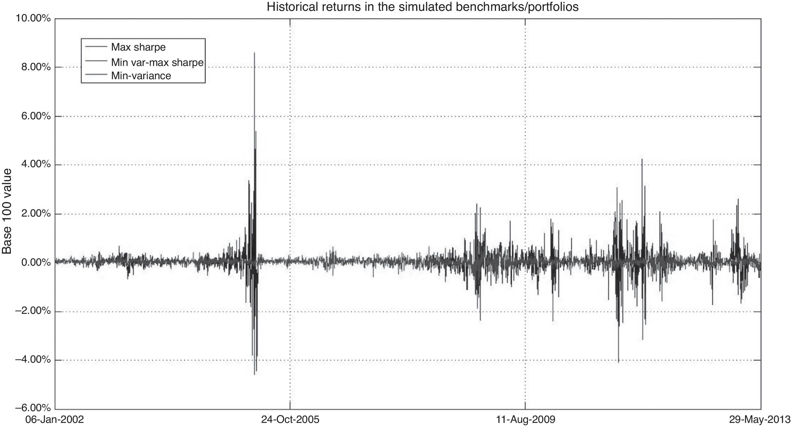

Fig. 3 Historical volatility (standard deviation) in the three simulated portfolios. Source: Data from simulations.
Even though we calculated the observed daily Sharpe ratio (5) and noted a more volatile behavior in the Max Sharpe portfolio (shown in Fig. 4), we performed a one-way ANOVA test in order to determine if the efficiency levels were equal. Table 3 gives the results of the test. In the upper panel of that table we present the one-way ANOVA test for the entire simulation values and, in the lower one, we show the results of a rolling ANOVA test by year, noting the robustness of our results by the fact that the conclusion holds in different time periods such as the years of 2007-2009. The years of the most resent economic and financial crisis.

Table 3 ANOVA test of the observed Sharpe ratios.
| One-way ANOVA test (entire simulation) | |||||
|---|---|---|---|---|---|
| Source | Squared sum | Degrees of freedom | Mean squared | F | Prob > F |
| Columns | 2.540884373 | 2 | 1.270442186 | 0.210683909 | 81.00% |
| Error | 51919.04433 | 8610 | 6.030086449 | ||
| Total | 51921.58521 | 8612 | |||
| One-way ANOVA test by year | |||||
|---|---|---|---|---|---|
| Year | Prob > F | Year | Prob > F | Year | Prob > F |
| 2002 | 82.67% | 2006 | 99.99% | 2010 | 95.84% |
| 2003 | 99.23% | 2007 | 99.93% | 2011 | 98.56% |
| 2004 | 90.13% | 2008 | 94.32% | 2012 | 82.16% |
| 2005 | 57.14% | 2009 | 83.98% | 2013 | 82.16% |
Source: Data from own simulations.
In order to see if this result holds, we performed a one-market factor model by assuming that the min variance portfolio was the market benchmark and by testing the null hypothesis H 0 : α ≠ 0. If this hypothesis holds, the Max Sharpe or the MV-Max Sharpe benchmarks would be a more efficient portfolio, suggesting its use as a better strategy benchmark for the IPS of the SIEFOREs. In order to deal with autocorrelation and heteroskedasticity, we calculated the standard errors by using the Newey-West (1987) consistent covariance matrix. This test is very important by the fact that it gives a hint if the Max Sharpe or the MV-Max Sharpe benchmarks have an expected out performance (expected alpha) than the min variance one i.e. if the observed Jensen's alpha in the model is statistically significant, we will find evidence against the min variance index (used as market factor in the model) by the fact that the expected value of this index lead to poorer results than the Max Sharpe one. We present the results in Table 4 and we found no significant alpha in the model, suggesting that neither the Max Sharpe nor the MV-Max Sharpe benchmarks lead to any outperformance. Why? Because the alpha value is equal to zero21 and is not significant and the beta value is around 1 and significant, suggesting a similar performance between benchmarks. For this reason, we find evidence that supports the min variance is a preferable benchmark by the fact that it has more flexible theoretical parameters than the other two and its mean-variance efficiency is practically the same to the other two cases.
Table 4 Jensen's alpha test for the Max Sharpe benchmark as active portfolio and the Min variance as market factor.
| Coefficient | Value | Newey-West std. error | Newey-West t. value | Probability |
|---|---|---|---|---|
| Max Sharpe/Min variance Jensen's alpha test | ||||
| α | 0.0001 | 0.0012 | 0.0469 | 39.8468% |
| β | 1.0039 | 0.0114 | 88.4374 | 0.0000% |
| R -squared | 0.9562 | Adj. R -squared | 0.9559 | |
| F stat. | 2924.4909 | Prob. > F | 0.0000% | |
| MV-Max Sharpe/Min variance Jensen's alpha test | ||||
| α | 0.0000 | 0.0006 | −0.0047 | 39.8903% |
| β | 1.0019 | 0.0057 | 175.0523 | 0.0000% |
| R -squared | 0.9882 | Adj. R -squared | 0.9881 | |
| F stat. | 11233.8215 | Prob. > F | 0.0000% | |
Source: Data from own simulations.
From Table 4, we observed that the value of the beta in both regressions is closer to one. For this reason we decided to run, in the same regression model of Table 4, the Huberman and Kandel's (1987) spanning test. With this result we tested the null hypothesis H 0 : α = 0, β = 1, presenting our results in Table 5. The values suggest that the null holds, concluding that the min variance benchmark can be used as a substitute of the Max Sharpe portfolio. If we use the min variance portfolio instead of the Max Sharpe we will arrive at a similar performance.
Table 5 Huberman and Kandel's (1987) spanning test for the Max Sharpe benchmark as active portfolio and the Min variance as market factor.
| Coefficient | Value | Newey-West std. error | Newey-West t. value | Probability |
|---|---|---|---|---|
| Max Sharpe/Min variance spanning test | ||||
| α | 0.0001 | 0.0012 | 0.0469 | 39.8468% |
| β | 1.0039 | 0.0114 | 88.4374 | 37.6396% |
| R -squared | 0.9562 | Adj. R -squared | 0.9559 | |
| F stat. | 2924.4909 | Prob. > F | 0.0000% | |
| MV-Max Sharpe/Min variance spanning test | ||||
| α | 0.0000 | 0.0006 | −0.0047 | 39.8903% |
| β | 1.0019 | 0.0057 | 175.0523 | 37.7090% |
| R -squared | 0.9882 | Adj. R -squared | 0.9881 | |
| F stat. | 11233.8215 | Prob. > F | 0.0000% | |
| Max Sharpe/Min variance spanning test | ||||
| α | 0.0001 | 0.0012 | 0.0469 | 39.85% |
| β | 1.0039 | 0.0114 | 88.4374 | 37.64% |
| R -squared | 0.96 | Adj. R -squared | 0.96 | |
| F stat. | 2924.49 | Prob. > F | 0.00% | |
Source: Data from own simulations.
Thus far we have found that, for this specific set of financial assets (markets) and given the investment level restrictions or legal constraints in Table 2, the simulated benchmarks have a similar performance. Despite this result, we want to focus our attention on the risk profile. Following Figure 2 and as theoretically expected, it is observable that the Max Sharpe and the MV-Max Sharpe benchmarks were exposed to higher risk levels. With this hint we answer the question "How much risk is acceptable in order to prefer one benchmark from another?" In order to answer it we performed a first test with the observed max drawdown or potential loss level in each benchmark. To do so, we focused on the daily −0.7% total portfolio Value at Risk constraint given in CONSAR (2012). To compare the risk exposure in the simulated benchmarks, we performed three tests. First we used the −0.7% limit (in daily basis) to count the number of days when the simulated benchmarks had a lower Δ%(pt) value than the given threshold. We compared this count with a λ=2.871⋅5%=143.5≈144 parameter in order to determine if the number of days with a return value under the threshold was big enough in the simulation.22 The results are shown in Table 6 and even though all the simulated benchmarks fit the λ parameter, the min variance benchmark had an observable lower risk level (just 5 days with a return lower than −0.7%). As a second test, we used the same −0.7% expected loss limit and compared it with the observed Conditional VaR (CVaR23) calculated with a 95% confidence interval and 10,000 slices between the [95%, 100%] interval. We present a resume of the daily observed CVaR values in Table 7 and historical CVaR values in Figure 5. As noted both the Max Sharpe and the MV-Max Sharpe benchmarks do not fit with the −0.7% daily CVaR threshold value and hence, their use seems to be questionable in the risk exposure profile.
Table 6 Shortfall −0.7% threshold value count and risk exposition.
| Benchmark | Poisson pdf critical value | Poisson Statistic (days with Δ% <−0.7% count) |
|---|---|---|
| Min Variance | 164 | 5 |
| Max Sharpe | 164 | 103 |
| MV-Max Sharpe | 164 | 40 |
Source: Data from own simulations.
Table 7 CVaR values and backtest with the −0.7%% threshold value.
| CVaR (%) values resume | |||||
|---|---|---|---|---|---|
| Benchmark | Mean value | Median | Std. dvn. | Min | Max |
| Min variance | −0.2401% | −0.1944% | 0.1225% | −0.6067% | −0.1185% |
| Max Sharpe | −0.2781% | −0.2142% | 0.1721% | −0.8634% | −0.1185% |
| MV−Max Sharpe | −0.2781% | −0.2142% | −0.2142% | −0.8634% | −0.1185% |
| CVaR Poisson count: CVaR < threshold | ||
|---|---|---|
| Benchmark | Poisson pdf critical value | Poisson statistic |
| Min Variance | 144 | 0 |
| Max Sharpe | 144 | 221 |
| MV-Max Sharpe | 144 | 221 |
Source: Data from own simulations.

In order to confirm this result we performed a stress test by using the first principal component24 as common covariance factor. We decided to use this component by the fact that the use of any financial or economic factor sensitivity needs either a previous theoretical support or a universal application to all the asset types used. The first principal component, as accepted in the portfolio management literature, is a latent factor that creates a common covariance between assets or asset types, therefore, its use is suggested as a proxy of the common factor in the simulated portfolios.
We present the results of our stress test, measuring the impact of a −1 to −6 sigma movement in the first principal component in a one year time frame. As noted, the Min variance portfolio has a lower shortfall than the other two cases with a shortfall of −0.1676% if the first principal component has a −6 sigma move (a value notably lower than the −0.7% daily threshold).
Therefore, the results presented thus far suggest that the min variance benchmark leads to a similar performance than the Max Sharpe and MV-Max Sharpe ones with a significantly lower market risk (expected shortfall or Value at Risk) exposure.
As another benchmark quality criteria for the min variance portfolio, we decided to review the representativeness of the six markets of interest in the three simulated benchmarks. We did this with the aforementioned Engle and Granger cointegration test by using the price (P t ) time series of each simulated benchmark as dependent variable and the six market benchmarks of Table 2 as regressors. The results of this test are shown in Table 9 for the min variance benchmark and, in Table 10 for the Max Sharpe and in Table 11 for the MV-Max Sharpe one.25
Table 8 Stress tests of the simulated portfolios using the 1st principal component.
| Portfolio (index)/yearly σ movement | −1σ movement in 1st principal component | −2σ movement in 1st principal component | −3σ movement in 1st principal component |
|---|---|---|---|
| Min variance | −0.0279% | −0.0559% | −0.0838% |
| Max Sharpe | −0.1480% | −0.2961% | −0.4441% |
| MV-Max Sharpe | −0.1480% | −0.2961% | −0.4441% |
| Portfolio (index)/yearly s movement | −4σ movement in 1st principal component | −5σ movement in 1st Principal component | −6σ movement in 1st principal component |
|---|---|---|---|
| Min variance | −0.1118% | −0.1397% | −0.1676% |
| Max Sharpe | −0.5922% | −0.7402% | −0.8882% |
| MV-Max Sharpe | −0.5922% | −0.7402% | −0.8882% |
Source: Data from own simulations.
Table 9 Min variance benchmark's Engle and Granger test.
| Auxiliary regression values | ||||
|---|---|---|---|---|
| Market | Coefficient | Std. error | t -Stat. | Probability |
| α | 0.0000 | 0.0000 | 2.90 | 0.37% |
| Mex-Government | 0.5192 | 0.0156 | 33.21 | 0.00% |
| Mex-Corporate | 0.2710 | 0.0202 | 13.41 | 0.00% |
| Mex-Equity | 0.0599 | 0.0008 | 71.42 | 0.00% |
| World Fixed-Income ex MBS | 0.0448 | 0.0010 | 43.70 | 0.00% |
| World Equity | 0.0012 | 0.0011 | 1.05 | 29.41% |
| Commodities | 0.0100 | 0.0007 | 14.71 | 0.00% |
| Adj. R -squared | 0.91 | RMSE | 0.0005 | |
| Durbin-Watson | 2.05 | Hannan-Quinn | −35830.99 | |
| Residual's one-step cointegration test | ||||
|---|---|---|---|---|
| Dependent variable | Critical value | Statistic | P value | Test conclusion |
| Min variance bmk | −4.9931 | −54.8188 | 0.10% | Cointegrated |
Source: Data from own simulations.
Table 10 Max Sharpe benchmark's Engle–Granger test.
| Max Sharpe benchmark's Engle-Granger test | ||||
|---|---|---|---|---|
| Auxiliary regression values | ||||
| Market | Coefficient | Std. error | t -Stat. | Probability |
| α | 0.0001 | 0.00 | 0.68 | 49.72% |
| Mex-Government | 0.4566 | 0.16 | 2.84 | 0.46% |
| Mex-Corporate | 0.1557 | 0.21 | 0.75 | 45.40% |
| Mex-Equity | 0.0615 | 0.01 | 7.12 | 0.00% |
| World Fixed-Income ex MBS | 0.1247 | 0.01 | 11.82 | 0.00% |
| World Equity | 0.0080 | 0.01 | 0.70 | 48.46% |
| Commodities | 0.0173 | 0.01 | 2.47 | 1.34% |
| Adj. R -squared | 0.11 | RMSE | 0.0048 | |
| Durbin-Watson | 2.13 | Hannan-Quinn | −22444.40 | |
| Residual cointegration test | ||||
|---|---|---|---|---|
| Dependent variable | Critical value | Statistic | P value | Test conclusion |
| Max Sharpe bmk | −4.9931 | −57.14162 | 0.10% | Cointegrated |
Source: Data from own simulations.
Table 11 MV-Max Sharpe benchmark's Engle–Granger test.
| Auxiliary regression values | ||||
|---|---|---|---|---|
| Market | Coefficient | Std. error | t -Stat | P value |
| α | 0.0000 | 0.0000 | 0.8661 | 38.65% |
| Mex-Government | 0.4874 | 0.0829 | 5.8780 | 0.00% |
| Mex-Corporate | 0.2131 | 0.1072 | 1.9888 | 4.68% |
| Mex-Equity | 0.0608 | 0.0045 | 13.6692 | 0.00% |
| World Fixed-Income ex MBS | 0.0853 | 0.0054 | 15.6895 | 0.00% |
| World Equity | 0.0045 | 0.0059 | 0.7755 | 43.81% |
| Commodities | 0.0136 | 0.0036 | 3.7769 | 0.02% |
| Adj. R -squared | 0.2854 | RMSE | 0.0024 | |
| Durbin-Watson | 2.1210 | Hannan -Quinn | −26251.6012 | |
| Residual cointegration test | ||||
|---|---|---|---|---|
| Dependent var | Critical value | Statistic | P value | Test conclusion |
| Max Sharpe bmk | −4.9931 | −56.9081 | 0.10% | Cointegrated |
Source: Data from own simulations.
As noted with the Hannan-Quinn criterion, the min variance benchmark has a better fit than the Max Sharpe and MV-Max Sharpe ones, suggesting that this benchmark is more representative of the six markets of interest than the latter. In the min variance benchmark, only the world equity markets was the type of asset that did not explain the performance of the benchmark (with a probability of 29.41%). If we follow this analysis in the Max Sharpe and MV-Max Sharpe benchmarks we note that the Mexican corporate bonds (at a 5% significance level), along with the world equity markets, do not explain its performance, reducing its market representativeness.
Therefore, at this point, even if we had found that the min variance benchmark leads to a similar performance than the Max Sharpe one, we preferred the use the former by the fact that the risk exposure and the markets representativeness is better than the other two cases.
Finally, in search for the causes of these results, we found an interesting turnover result. To give a first hint,26 we present, in Table 12, a statistical summary of the observed investment levels in each simulated portfolio. As noted, despite the fact that the benchmarks showed the same concentration level (a normalized Herfindahl-Hirsch index value of 0.32), their individual mean investment level in each market is different, giving an explanation of the different performance, observed risk level and market representativeness results in each benchmark.
Table 12 Investment levels statistical resume for the simulated benchmarks.
| Statistic | Mex-Government | Mex-Corporate | Mex-Equity | World Fixed-Income ex MBS | World Equity | Commodities |
|---|---|---|---|---|---|---|
| Min variance portfolio investment levels | ||||||
| Mean | 57.43% | 34.94% | 3.27% | 2.67% | 0.87% | 0.82% |
| Stdv. | 12.08% | 13.33% | 0.00% | 1.91% | 0.77% | 0.01% |
| Max | 85.46% | 42.63% | 3.27% | 8.98% | 5.87% | 0.97% |
| Min | 51.00% | 8.17% | 3.27% | 1.63% | 0.65% | 0.82% |
| Median | 51.00% | 42.29% | 3.27% | 1.63% | 0.65% | 0.82% |
| Min variance normalized Herfindahl-Hirsch index | 0.32 | |||||
| Max Sharpe portfolio investment levels | ||||||
| Mean | 54.99% | 33.89% | 3.76% | 4.67% | 1.31% | 1.38% |
| Stdv. | 8.83% | 11.94% | 2.36% | 5.25% | 1.49% | 1.56% |
| Max | 85.46% | 42.63% | 37.73% | 19.35% | 12.43% | 10.00% |
| Min | 51.00% | 8.17% | 3.27% | 1.63% | 0.65% | 0.82% |
| Median | 51.00% | 39.36% | 3.27% | 1.63% | 0.65% | 0.82% |
| Max Sharpe normalized Herfindahl-Hirsch index | 0.32 | |||||
| MV-Max Sharpe portfolio investment levels | ||||||
| Mean | 56.22% | 34.41% | 3.51% | 3.67% | 1.09% | 1.10% |
| Stdv. | 7.18% | 9.07% | 1.18% | 3.25% | 0.93% | 0.78% |
| Max | 80.40% | 42.63% | 20.50% | 13.72% | 7.24% | 10.00% |
| Min | 51.00% | 8.17% | 3.27% | 1.63% | 0.65% | 0.82% |
| Median | 51.00% | 39.41% | 3.27% | 1.63% | 0.65% | 0.82% |
| MV-Max Sharpe normalized Herfindahl-Hirsch index | 0.32 | |||||
Source: Data from own simulations.
As noted in this table, the Max Sharpe and MV-Max Sharpe portfolios invested less in the Mexican corporate bonds and more in Mexican Government bonds, world equity markets and commodities. Table 13 shows the statistical summary of the six markets that conform the investment universe and, as noted, the world equity markets and commodities are among the riskiest assets, giving another explanation of the difference in the risk levels of the simulated benchmarks.
Table 13 Statistical table of the six markets of interest.
| Statistic | Mex-Government | Mex-Corporate | Mex-Equity | World Fixed-Income ex MBS | World Equity | Commodities |
|---|---|---|---|---|---|---|
| Mean | 0.03% | 0.04% | 0.06% | 0.04% | 0.02% | 0.02% |
| Stdv. | 0.13% | 0.10% | 1.32% | 0.86% | 0.95% | 1.36% |
| Max | 1.92% | 1.15% | 10.44% | 8.11% | 5.88% | 8.96% |
| Min | −1.40% | −0.95% | −7.27% | −7.66% | −8.03% | −7.20% |
| Median | 0.03% | 0.04% | 0.11% | 0.02% | 0.04% | 0.00% |
Source: Data from own simulations.
From the results of the investment levels in Table 12, we also studied the turnover levels and we noted that the Max Sharpe benchmark has the highest level by the fact that almost all the financial markets (or assets) had a higher standard deviation level in the daily investment level (i.e. there was a lot of rebalancing). Therefore, when we calculated a mean of the six standard deviations in the Max Sharpe benchmark, we arrived at a mean turnover of a daily 6.6%, a value that is higher than the daily 0.22% (20% quarterly) level suggested by Bailey (1992). For the case of the min variance benchmark, we found a more suitable value of 0.52%.
Conclusions
In the present paper we propose the use of the minimum variance portfolio (or min variance portfolio) as weighting method for a performance benchmark of the defined contribution (DC) pension funds in Mexico (also known as SIEFOREs). To do this, we proved as true the next hypothesis "The minimum variance benchmark of the SIEFOREs' IPS is as mean-variance efficient as the Max Sharpe and the MV-Max Sharpe ones but preferable than these by its risk exposure and representativeness". We achieve this by assuming that all of the SIEFOREs in Mexico, by following CONSAR's (2012) legal constraints, invest in all of the next financial assets or markets (benchmarks given in parentheses):
Mexican Government bonds (Valmer Gubernamental index),
Mexican corporate bonds (Valmer Corporativo index),
Mexican stocks (IPC index),
World investment grade sovereign and corporate bonds - ex MBS - (Citigroup WorldBIG index),
World equities (MSCI world index) and
Commodities (DJ-UBS commodities index).
We did so by using MXN based values and the legal constraints (investment Policy statement or IPS) given in CONSAR (2012).
In order to test our proposal, we compared the minimum variance (min variance) benchmark against the theoretical reference given with the tangency or Max Sharpe portfolio and a linear combination of the Min variance and the latter as Amenc et al. (2012) suggest.
We preferred to use the min variance benchmark as weighting method instead of a market cap one of all the traded SIEFOREs by the fact that there could be a concentration in the investment levels with this approach (i.e. some SIEFORES are notable bigger than others) and the use of the proper investment restrictions is an issue to be determined in future research.
We also chose this sort of quantitative weighting method because the public price (that leads to the market-cap level) of a SIEFORE is the result of its IPS execution and because a quantitative method is less criticized (theoretically speaking) than the market cap in its mean-variance efficiency.27
Therefore, by following this rationale, we performed two discrete event simulations (for both simulated benchmarks) with daily data of the six aforementioned indexes, from January 3, 2002 to May 27, 2013.
By using the Sharpe (1966) ratio and the Jensen's (1968) alpha in a one factor market model (the min variance benchmark as market factor), we found that the performance of the simulated benchmarks was statistically equal. Complementary to this finding, by using Huberman and Kandel's (1987) spanning test, we noted that the min variance portfolio could be used as a good proxy of the Max Sharpe's performance with the min variance benchmark as an appropriate substitute of the latter.
With this in mind, we decided to focus our attention on the risk level through the expected shortfall (or maximum drawdown) and daily CVaR values in each benchmark. We also tested the representativeness that each benchmark or asset type had from the financial assets (financial markets) that conform the benchmark.
The results of the maximum drawdown and CVaR tests show that the min variance benchmark, as theoretically expected, had a lower risk exposure than the Max Sharpe ratio and MV-Max Sharpe ones. Complementary to this, as another benchmark quality criteria, an Engle and Granger test observed that even though the simulated benchmarks were cointegrated with the six markets of interest the min variance portfolio had the highest representativeness of all.
As a final test of the min variance benchmark's quality against the Max Sharpe one, we found that the former had more acceptable turnover levels (4.68% daily mean standard deviation in the observed investment levels in each market) than the Max Sharpe (5.24%).
Therefore, by observing that the min variance benchmark leads to the same performance than the Max Sharpe and MV-Max Sharpe ones and by the fact that it had a lower risk exposure and a better market representativeness than these, we strongly support the use of a min variance weighting method to calculate a benchmark that measures the performance of the all the SIEFORE's in Mexico and also to use it as a benchmark weighting method in other private pension funds (either DC or Defined Benefit ones).
At this point, we also recommend CONSAR to consider this weighting method to calculate and make public the daily values of a strategy benchmark that could be used (either by pension fund managers or by investors) to measure the performance of SIEFOREs and other sort of private pension funds.
Some of the drawbacks of the present paper that must be noted are the fact that we used a specific and closed data set given with the six benchmarks of Tables 1 and 2 . With this in mind, we recommend, for further research, to test directly other sorts of benchmarks to incorporate the effect of different covariance among assets. In a complementary manner, we must contemplate the use of other sorts of investment restrictions (different to the CONSAR (2012) rules) to see if the conclusions that we present hold.
Therefore, the present paper gives the results of our first findings, observing that the determination of proper investment levels, the test of the min variance portfolio against other weighting methods, the use of different data sets or the determination of other investment level restrictions are tasks in current research, being the present one of the first studies on the use of minimum variance portfolios as benchmarks in pension funds of emerging markets and Mexico.


