Three discount methods for valuing projects and the required return on equity

 

Tres métodos de descuento para valuar proyectos y la tasa requerida de rendimiento para el capital accionario

 

Marc B.J. Schauten

 

Erasmus School of Economics. E–mail: schauten@ese.eur.nl

 

Fecha de recepción: 26/04/2011.
Fecha de aceptación: 29/08/2011.

 

Abstract

In this paper we discuss the required return on equity for a simple project with a finite life. To determine a project's cost of equity, it is quite common to use Modigliani and Miller's Proposition II (1963). However, if the assumptions of MM do not hold, Proposition II will lead to wrong required returns and project values. This paper gives an example of how the cost of equity should be determined in order to obtain correct valuations. The methods we apply are the Adjusted Present Value method, the Cash Flow to Equity method and the WACC method.

Keywords: Proposition II, net present value, APV, CFE, WACC.

JEL classification: G12; G31; G32; H43.

 

Resumen

En este artículo analizamos el rendimiento requerido para el capital accionario en un proyecto simple con vida finita. Es muy común el uso de la Proposición II de Modigliani y Miller (1963) para determinar el costo del capital accionario de un proyecto. No obstante, si los supuestos de MM no se mantienen, la Proposición II llevará a rendimientos requeridos y valores del proyecto erróneos. Este trabajo brinda un ejemplo de cómo el costo del capital accionario puede determinarse de forma que se obtengan valuaciones correctas. Los métodos que aplicamos son el del Valor Presente Ajustado, el del Flujo de Efectivo a Capital y el método del CPPC.

Palabras clave: proposición II, valor presente neto, APV, CFE, CPPC.

Clasificación JEL: G12; G31; G32; H43.

 

Introduction

The value of a project can be calculated using the 'Adjusted Present Value' (APV) method, the 'Cash Flow to Equity' (CFE) method and the 'Weighted Average Cost of Capital' (WACC) method. According to the APV–method the value of a project equals the present value of the expected cash flows as if the project is all equity financed plus the present value of the tax shields (PVTS) due to debt financing.¹ The CFE–method discounts the after–tax cash flows to the equity holders at the cost of equity. The WACC–method discounts the after–tax cash flows at the weighted average cost of equity (E) and debt (D). Two versions of the WACC–method can be identified. The first version calculates the after–tax cash flows as if the project is all equity financed ('Free Cash Flows' or 'FCFs'. The advantage of debt financing is expressed in a lower discount rate. The second version, as presented by Ruback et al. (2002) discounts the expected after–tax cash flows ('Cash Flows to Capital' or 'CFC's) at a weighted average cost without taking the tax advantage of debt financing into account.

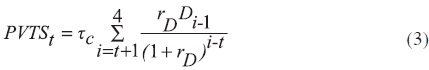
In this paper we focus on the valuation of a fictitious project with a finite life. We apply the APV–method, the CFE–method and the WACC–method. The project is financed with both E and D. The cost of equity (r_E), which needs to be determined in the last two methods, depends on both the business risk and the financial risk. The higher a project's degree of leverage, the higher the financial risk for the equity holders. Often, in calculating r_E, Modigliani and Miller's 'proposition II' is applied. Miller and Modigliani's well–known 'proposition II' states that (1963, equation 12c, p. 439):

where r_U is the cost of equity assuming 100% equity financing,² τ_c equals the corporate tax rate, r_D³ equals the cost of debt and E and D denote the market values of equity and debt. Important assumptions used by MM in their derivation are that tax savings are discounted at r_D debt is perpetual and the expected cash flows are perpetual with a growth rate of zero. However, the cash flows of our fictitious project are not perpetual and its leverage is not constant over time, such that application of MM II would lead to incorrect required returns which would result in incorrect project values. When valuing projects (and companies) this is often overlooked or ignored for simplicity reasons. This paper pursues an alternative approach for the determination of r_E, considering finite projects and a predetermined amount of debt (see Inselbag and Kaufold, 1997⁴). The suggested approach leads to valuations that yield the same results with all of the three valuation methods. Given the assumptions, these valuations are correct and consistent. When applying MM II to the project, this is (unfortunately) not the case.

This introduction is the first section. Section two presents the project. Section three determines the value of the project using the APV–, CFE–, and WACC–method. Section four gives a brief overview of the existing literature on the valuation of the tax shield and the discount rate of the tax shield in particular. This discount rate partially determines r_E. Finally, section five provides a summary.

 

Project X

The project to be valued, project X, requires an initial investment of € 230 million at t=0. This amount is divided into a € 200 million investment in tangible fixed assets (TFA) and a € 30 million investment in working capital (WC). To finance the investment, € 150 million of debt is issued at t = 0. The maturity of the (bullet) loan is 4 years. The loan pays 8% interest (r_D = 8%) at the end of each year. The market value of debt equals € 150 million at the beginning of each year. The residual of the initial investment (€ 230 million – € 150 million = € 80 million) is financed with equity. The corporate tax rate τ_c is 40%. The forecasted profit– and loss accounts, balance sheets and cash flow statements of the project are reported in Table 1.

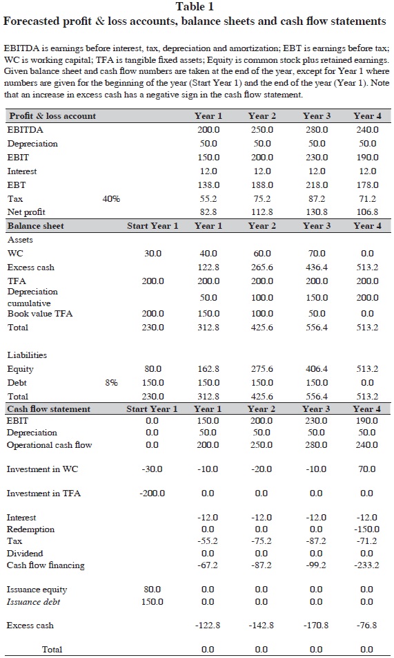
Note that dividends in the cash flow statements are set to zero. Actual dividends are probably higher than zero. The zeros could subsequently be interpreted as wrong and of influence on the outcome of the valuation. This —however— is not the case. The item dividend is —as well as the item excess cash in the balance sheets— ignored when we calculate the free cash flows needed for the valuations in The AVP and WACC methods. The value of a project is determined by the present value of free cash flows generated by the project. This free cash flow is not influenced by dividend policy. Whether the actual cash generated is invested in a zero NPV savings account and paid out later or paid out directly as dividend is irrelevant for the valuation of the project. Of course, if one applies the ECF method, then the most convenient way to calculate the equity cash flow is to assume that the net cash generated is each year directly paid to the shareholders as dividend. It is of course possible to incorporate the ECFs (see CFE method) in the cash flow statement and the balance sheet. This would of course increase the 'cash (out)flow financing' item in the cash flow statements and would decrease 'equity' in the balance sheets. But it will not influence the outcomes of the valuations.⁵

 

The APV, CFE and WACC methods

The APV method

According to the APV method, the value of the project at time t (V_L,t = E_t + D_t) equals the value of the project as if it was all–equity financed plus the present value of the tax shields at time t, PVTS_t:

The project value assuming 100% equity financing at time t equals:

where cash flow_i denotes the after–tax cash flow at time i and r_u denotes the cost of capital as if the project was all–equity financed (= free cash flow).

The present value of the tax savings at time t is:

where τ_c denotes the corporate tax rate and r_D equals the cost of debt.

The FCF equals the operational cash flow minus the investment in working capital and TFA minus taxes as if the project is 100% equity financed. For example, at the end of year 1 (t = 1) the FCF equals 200 – 10 – (40% x 150) = 130.

Table 2

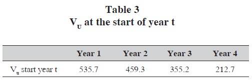
V_u at t = 0 then equals:⁶

This way, we can determine V_u at the beginning of each year. For example, V_u at the beginning of year 4 equals:

Table 3 reports the values of project X at the beginning of the years 1–4, assuming that the project is all–equity financed.

The PVTS at the beginning of year 1 equals (see Equation 3):

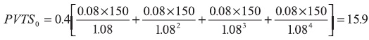
The PVTS at t=0 is the present value of the tax shields due to debt financing in year 1–4. The interest payment at the end of each year is 12. Compared to all–equity financing, the tax payment is 0.4 x 12 (=τ_c x interest) lower per year. Since the amount of debt is independent of the value of the project, the tax savings and the interest payments are assumed to have the same risk profile. Therefore, the present value of tax savings is calculated using the discount rate r_D (= 8%).

This way, we can determine PVTS at the beginning of each year. For example, the PVTS at the beginning of year 4 equals:

Table 4 reports the values of project X at the beginning of the years 1–4.

The total project value (V_L = V_U + PVTS) at the beginning of year 1 equals 551.6 (=535.7 + 15.9). The market value of equity at the beginning of the first year equals 551.6 minus the market value of debt: 551.6–150=401.6. The equity providers initially invested 80.0 (=230–150), while the market value equals 401.6. This gives a net present value (NPV) of the project for the equity holders of 401.6–80.0=321.6.⁷

The CFE method

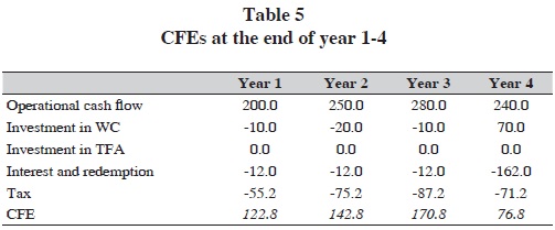
The market value of equity at the beginning of year 1–4 can also be determined by discounting the CFEs with r_E as discount rate. The CFE in year t equals the operational cash flow minus the investment in working capital and TFA minus interest (and redemption) paid minus the actual corporate taxes paid, all in year t. Table 5 reports the CFEs for year 1–4. For example, the CFE at the end of year 1 equals: 200–10–12–55.2= 122.8. The CFE at the beginning of year 1 equals the deposit of € 80 million to partially finance the investment expense of € 230 million at t=0.

R_E is determined by the business risk of the project and the financial risk due to debt financing. As mentioned before, the business risk determines R_U and equals 10% in the year 1–4. Financial risk for the equity holders is determined by the relative amount of debt. The leverage varies over the lifetime of the project; see Table 4. For example, the D/E ratio is 37% (=150/401.6) at the beginning of year 1 and 223% (= 150 / 67.2) at the beginning of year 4. Because the financial risk is fluctuating, r_E is fluctuating as well. Following Inselbag and Kaufold (1997) we derive an 'adjusted proposition II' for r_E. Let's start with the basic balance sheet identity. The total value of project X at time t equals:

The value increase required by the equity– and debt holders over period t (for example from t = 0 to t = 1) equals D_t(r_D)+ E_t(r_E,t). This value increase equals V_u,t(r_u)+PVTS_t(r_D). V_u yields a return equal to r_U and, as the PVTS faces the same risk as the debt, the PVTS yields a return equal to r_D:

From (5) it follows, after rearranging, that⁸:

Equation (6) reflects the general formula for the required return on equity under the assumption that the discount rate for the tax shields is equal to r_D. Only if the PVTS of a project is equal to τ_c x D_t=0 equation (6) can be rewritten as proposition II of MM (MMII).⁹ For project X, using equation (6) r_E,t can be calculated for the years 1 to 4. This requires entering the computed values resulting from the APV–method (see Table 4) in (6). For year 1, this yields a required rate of return on equity of:

Table 6 reports the r_Es for year 1–4. We notice an increase in R_E from 10.668% in year 1 to 14.334% in year 4. The required return increases, because of an increase in the ratio (D – PVTS) / (E).

Naturally, R_E in year t equals the CFE_t (see Table 5) plus the value change of equity in year t, divided by the market value of equity at t–1 (see Table 4). For example, R_E,1 equals [122.8 + (321.6 – 401.6)] / 401.6 = 10.668% and r_E,4 equals [76.8 + (67.2 – 213.8)] / 213.8 = 14.334%.

The value of equity at the beginning of year 1 is the present value of the expected ECFs:

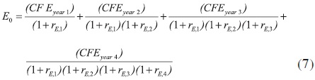
If we insert in the numbers from Table 5 and Table 6 we find:

And the value of equity at the beginning of, for example, year 4 equals:

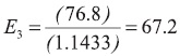
The computed equity values match the values resulting from the APV–method (see Table 4). However, this would not have been the case if we would have used MM II instead of Equation 6.¹⁰

The WACC method

We can identify two versions of the WACC method. The first version calculates the after–tax WACC.¹¹ This version is most commonly used. The second version uses the before–tax WACC.

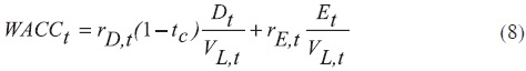
Version 1. The project value can be determined by discounting the expected FCFs with the WACC_{after taxes}. The market value of equity at time t then equals the project value at time t minus the debt value at time t. The tax advantage from debt financing is expressed in the discount rate. The WACC for period t equals the weighted average of r_D,t after taxes and r_E,t:

Using the outcomes from the APV–approach, the WACC can easily be determined. Table 7 reports the market values of equity and debt and the accompanying required returns per year.

The WACC for year 1 then equals:

And the WACC for year 4, for example, equals:

The value of the project (E + D) at the beginning of year 1 equals:

If we insert the numbers from Table 2 and Table 7 we find:

The value of the project at, for example, the beginning of year 4 equals:

The computed project values match the computed values resulting from the APV–and the CFE–method.¹²

As an alternative to the WACC_{after taxes} the WACC_{before taxes} (or WACC^CFC) can be employed (see Ruback, 2002). Here we can assume that the tax savings are discounted at r_D, as we did before. In applications this can be simplified by assuming that the tax savings are discounted at r_u. Version 2a elaborates on the first situation and version 2b elaborates on the second.¹³

Version 2a. According to version 2a, the project value is calculated by discounting the free cash flow to equity (CFE) and the net cash flow to debt¹⁴ (CFD) at the WACC_{before taxes}. The difference with respect to version 1 is that the tax advantage is expressed in a higher cash flow instead of a lower discount rate;¹⁵ the sum of CFE and CFD —Cash Flow to Capital (CFC)— is higher than FCF. For example, the CFC in year 1 equals 122.8+12=134.8 and in year 4: 76.8+12+150=238.8, whereas the FCF in year 1 is 130 and 234 in year 4. Table 8 reports the CFC in year 1–4. (Table 8)

The WACC in period t equals the weighted average of r_Dt before taxes and r_E,t:

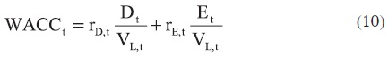
This gives a WACC in year 1 of:

And this gives a WACC in, for example, year 4 of:

Table 9 reports all WACC resulting from version 2a. These WACCs are higher than the WACCs under version 1, see Table 7.

Project value (E + D) at the beginning of year 1 equals:

Project value at, for example, the beginning of year 4 equals:

For valuations in practice, version 1 and 2a are not very useful. After all, the market values of equity, debt and r_E are required in order to calculate the WACC (after tax as well as before tax).

Version 2b. Following Ruback (2002), we can also use r_U instead of r_D as discount rate for the tax shield. This gives version 2 direct application possibilities, since calculating the PVTS by discounting the tax shield at r_U has the following effect on equation (5):

The value increase required by the equity and debt holders over period t equals the weighted average returns of V_U and the PVTS. As V_u and the PVTS yield the same return, the WACC_{before tax} is independent of the PVTS/V_U –ratio and is independent of the leverage ratio. After all, the amount of debt is one of the determinants of the PVTS. In other words, the WACC_{before taxes} is every year equal to r_u and does not depend on the capital structure.

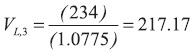
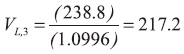
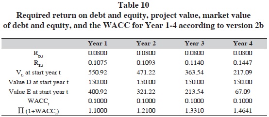
If the CFCs (see Table 8) are discounted at the WACC_{before taxes} (=10%), we obtain a market value of 550.92 at t=0. The market value of equity then is 550.92–150=400.92. The project values are reported in Table 10. Naturally, by applying the APV–method and the CFE–method, the same values are obtained. By applying the APV–method, we now use r_U as discount rate for the tax shield. By applying the CFE–method, the CFEs (see Table 8) are discounted at an adjusted r_E.¹⁶ It catches the eye that the market values turn out a little lower than they did in Table 7. This is not surprising as r_U (being the discount rate for the tax shield) is higher than r_D.

Summarizing, it can be stated that the WACC_{before taxes} can be directly used to determine the value of the project as long as the discount rate for the tax shields is equal to r_U. However, if r_D is used as discount rate for the calculation of the PVTS, applying the WACC–method would be tedious, as for both the WACC version the results of an APV calculation are required. So, if r_D is the discount rate for the PVTS, using the WACC–method is not very likely.¹⁷

 

The relation between the valuation of tax shields and the cost of equity

The required return on equity of a particular project (or firm) is among other things based on the chosen discount rate for the expected tax shields (r_TS) from interest bearing debt and the present value of the tax shields in relation to the unlevered value of the project.¹⁸ As long as the discount rate for the tax shields is lower than r_U, the relation between the required return on equity and the ratio PVTS to V_U is —ceteris paribus— negative. And if the discount rate is equal to r_U, there is no relation. The explanation for this is simple. The total cost of capital, i.e. the weighted average of r_E and r_D, is determined by the risk of the assets. As long as the level of risk of the PVTS is lower than the risk of V_U, the total risk of the assets reduces with PVTS. And if the level of risk of the PVTS is the same as the risk of V_U, the ratio PVTS to V_U is of no influence on the total risk of the assets and neither on r_E.

What can we say about the discount rate of the tax shields and the size of the PVTS? Miller and Modigliani (1963) assume that the risk free interest rate is the correct discount rate. And given non growing perpetual cash flows, the PVTS is equal to corporate tax rate times the amount of interest bearing debt.¹⁹ The relation between the cost of equity and leverage is then correctly reflected by (MM II). If the amount of debt is a growing perpetual with a constant growth rate g, then the PVTS as a percentage of the value of the project depends on g. And as long as the discount rate of the tax shields is lower than r_U, the required return on equity is negatively related to growth. The cost of equity decreases with the growth rate since the influence of growth on the PVTS is stronger than it is on Vu. If we assume that the discount rate of the PVTS is r_U, g is again irrevelevant for r_E. See Ehrhart and Daves (2002) for an overview of relations between the cost of capital and g.

If cash flows are not (growing) perpetuals, and if the discount rate for the tax shields is not equal to r_U, we need to know the level of risk (r_TS) and the PVTS in relation to firm value in order to determine r_E. (See Appendix C for a derivation of the general formula for r_E). The academic literature so far isn't unambiguous in its choice of the discount rate for the tax shields —and as a result of that it is unambiguous about the cost of equity and the WACC as well. In literature a distinction is often made between a fixed debt policy (the levels of debt are predetermined) and a situation where the level of debt is defined as a percentage of firm value. Analyzing the case of a fixed debt policy, Myers (1974) states that tax shields should be discounted at r_D, the debt holders' required rate of return. Luehrman (1997) also underwrites this discount rate. Harris and Pringle (1985), Ruback (2002), Kaplan and Ruback (1995), Brealey et al. (2008) and Berk and DeMarzo (2011) state that r_n is the appropriate discount rate for tax shields if firms follow a target debt ratio. They reason by saying that the systematic risk of the PVTS equals that of the operational activities of the firm/the project. Miles and Ezzel (1980) and Lewellen and Emery (1986) state that, when the companies follow a target debt ratio, r_D is the appropriate discount rate in the year in which the debt level is fixed, and r_U in all other years.

The PVTS could also be determined by taking the difference between the present value of the taxes paid by an unlevered firm (G_u) and an identical levered firm (G_l). Figure 1 depicts the total value of an unlevered and a levered firm (see Fernandez, 2004).²⁰ The focus then shifts to the appropriate discount rates for G_u and G_l respectively.²¹

We acknowledge that the choice of a correct discount rate for the tax shield still is a open issue. For now —following Brealey et al. (2008) and Berk and DeMarzo (2011)— we share the opinion that r_D is the correct discount rate when following a fixed debt policy, where the debt level is predetermined at the beginning of each year. The risk of the tax shield depends directly on the debt risk. This assumption is applied in the valuation of Project X as well (see The APV, CFE and WACC methods). The level of debt is predetermined as are the expected tax savings due to debt. However, if a target debt ratio is pursued, we recommend using r_U as the appropriate discount rate for the tax shield.²² Although Miles and Ezzel's (1980) method is more elegant, the differences in valuation are often minimal in practice.²³

 

Summary

By use of an example, we have shown in this paper that applying proposition II of MM (1963) can lead to incorrect values for projects with a finite life. The methods presented —the APV–method, the CFE–method and the WACC–method— then give different values for project X. When applying the CFE and WACC valuation methods, the cost of equity has to be determined correctly. If r_D is the discount rate for the tax shields, the equity holders' required return equals:

and does not equal proposition II of MM:

This MM relation is based on the assumption that the value of tax savings at t=0 equals the tax rate times the amount of debt. This does not hold for project X, as a result of which MM II is not applicable.

 

References

Arzac, E.R. and L.R. Glosten (2005). A reconsideration of tax shield valuation. European Financial Management (11): 453–461.         [ Links ]

Berk, J. and P. De Marzo (2011). Corporate Finance, 2nd edition, Boston: Prentice Hall.         [ Links ]

Brealey, R.A., S.C. Myers and F. Allen (2008). Principles of Corporate Finance, 9^th edition, New York: McGraw–Hill.         [ Links ]

Ehrhart, M.C. and P.R. Daves (2002). Corporate valuation: the combined impact of growth and the tax shield of debt on the cost of capital and systematic risk. Journal of Applied Finance (12): 31–38.         [ Links ]

Cooper, I.A. and K.G. Nyborg (2006). The value of tax shields IS equal to the present value of tax shields. Journal of Financial Economics (81): 215–225.         [ Links ]

Fernández, P. (2004). The value of tax shields is NOT equal to the present value of tax shields Journal of Financial Economics (73): 145–165.         [ Links ]

––––––––––(2005). Reply to Comment on 'The value of tax shields is NOT equal to the present value of tax shields. The Quarterly Review of Economics and Finance (45): 188–192.         [ Links ]

Fieten, P., L. Kraschwitz, J. Laitenberger, A. Löffler, J. Tham, I. Vélez–Pareja and N. Wonder. (2005). Comment on The value of tax shields is NOT equal to the present value of tax shields. The Quarterly Review of Economics and Finance (45): 184–187.         [ Links ]

Inselbag, I. and H. Kaufold (1997). Two DCF approaches for valuing companies under alternative financing strategies (and how to choose between them). Journal of Applied Corporate Finance 10(1): 114–122.         [ Links ]

Kaplan, S. and R. Ruback (1995). The valuation of cash flow forecast: an empirical analysis. Journal of Finance (50): 1059–1093.         [ Links ]

Lewellen, W.G. and D.R. Emmery (1986). Corporate debt management and the value of the firm. Journal of Financial Quantitative Analysis (21): 415–426.         [ Links ]

Luehrman, T. (1997). Using APV: a better tool for valuing operations. Harvard Business Review (75): 145–154.         [ Links ]

Miles, J.A. and J.R. Ezzell (1980). The weighted average cost of capital, perfect capital markets and project life: a clarification. Journal of Financial and Quantitative Analysis (15): 719–730.         [ Links ]

Myers, S.C. (1974). Interactions of corporate financing and investment decisions, implications for capital budgeting. Journal of Finance (29): 1–25.         [ Links ]

Modigliani, F. and M.H. Miller (1958). The cost of capital, corporation finance and the theory of investment. American Economic Review (48): 261–297.         [ Links ]

––––––––––(1963). Corporate income taxes and the cost of capital: a correction, American Economic Review (53): 433–443.         [ Links ]

Ruback, R.S. (2002). Capital Cash Flows: A Simple Approach to Valuing Risky Cash Flows. Financial management (Summer): 85–103.         [ Links ]

Schauten, M.B.J. and B. Tans 2009, Cost of Capital of Government's Claims and the Present Value of Tax Shields. Available at SSRN.         [ Links ]

 

Notes

¹ Since interest payments reduce taxable income. We ignore the value of other 'side effects'.

² rU is determined by the business risk of the project; a higher business risk implies a higher rU.

³ rD is the risk free interest rate in MM1963.

⁴ Inselbag and Kaufold (1997) value a fictitious firm with infinite cash flows instead of a finite project as we do.

⁵ Note that we should not make the mistake by adding possible expected 'returns' from the excess amount of cash to the (EBIT and) operational cash flow. The project would then be overvalued. An example: assume the expected cash flow at t = 1 is 110 and the opportunity cost of capital is 10%. The present value of this cash flow at t = 0 then is 100. It is wrong to add to this 100 the present value of the expected return during period 2 (e.g. the present value of 10% of 110). If you want to include this extra revenue then you should discount the expected cash flow at t = 2; 121 / 1.12 = 100.

⁶ t = 0 denotes the beginning of period 1, t = 1 the beginning of period 2 etc.

⁷ Obviously, the NPV for the debt holders is equal to zero. The market value of the loan at the beginning of year 1 equals the amount supplied by the providers of debt at t=0 (€ 150 million).

⁸ See appendix AI.

⁹ In their derivation MM assume equal interest payments per year. The annual tax shields are therefore the same every year: τc x rD x D. The PVTS at t=0 then equals (τc x rD x D) / rD = τc x D. The general formula for rE is derived in Appendix C.

¹⁰ If we would use the values obtained from the APV method (Table 4) to determine re in the years 1 to 4 according to MM II, we would find the following required returns for these years: 10.45%, 10.56%, 10.84% and 12.68%. If the CFEs in the years 1 to 4 (Table 5) would be discounted at these rates, the equity value at the beginning of year 1 would be 404.674 instead of 401.606.

¹¹ This method is also known as the 'textbook WACC'.

¹² For the years 1 to 4, WACC according to MMII amounts to, respectively, 8.91%, 8.73%, 8.35% and 7.24%. Here the computed APV–values (Table 4) are used to determine the required returns. This way, the total project value at t = 0 equals 554,830 instead of 551,606. The equity value at t=0 equals 404,830 (554,830 – 150) instead of 401,606.

¹³ A general formula for WACC_CFC can be derived by taking the weighted average of equation (C1) from Appendix C and r_D with the proportions equity to total value and debt to total value as weighting factors. The final result is: WACC_CFC = r_U – (r_U – r_TS)(PVTS/V_L).

¹⁴ Interest payments plus redemption minus newly issued debt.

¹⁵ Now the actual taxes are deduced instead of the taxes assuming all–equity financing.

¹⁶ It follows from (5'), after substituting V_L – PVTS for V_U and rearranging, that: See Appendix B.

¹⁷ The cash flow to capital (CFC) method as proposed by Ruback (2002) cannot be applied directly when a target capital structure is pursued. The WACC_{before taxes} indeed equals ry, but the CFCs cannot be determined directly. Namely, the yearly CFC partially depends on the amount of D. When a target capital structure is pursued the amount of D is a percentage of the unknown total project value at the beginning of each year.

¹⁸ Of course the return on equity is also positively influenced by the financial risk due to leverage. The higher the ratio D/E, the higher r_E.

¹⁹ If debt is not riskless we replace the riskless rate by the cost of debt.

²⁰ Although Fernáiidez's derivations leading to his final results are disputable, his conclusion that the present value of tax shields (PVTS) is equal to the difference between the present value of expected taxes paid by the unlevered firm (G_u) and the present value of expected taxes paid by the levered firm (G_l) is valid. For a discussion of the validity of the final results of Fernández (2004), see Fieten et al. (2005), Fernández (2005), Arzac and Glosten (2005) and Cooper and Nyborg (2006). According to Fernández (2004), the PVTS for non–growing perpetuities is equal to τD, where T is the tax rate and D is the market value of debt. PVTS for constant growth firms would be τDr_u/(r_u –g), where ru is the required return to unlevered equity and g is the constant growth rate.

²¹ See Schauten & Tans (2009) for a derivation of the cost of tax for the government. Note: the higher the leverage, the lower G_l, the higher Gu – G_l (= PVTS).

²² The WACC_{after taxes} then equals: WACC = r_u – (τ_cr_DD)/V_L (see Appendix B). If, at the beginning of each year, the project is 40% debt financed, the project value at t=0 equals 552,48. The amount of debt at t = 0 then equals 220,99 (40% of 552,48). The WACC_{before taxes} is not directly applicable, because the CFCs cannot be determined directly.

²³ The WACC_{after taxes} then equals: WACC = r_c –(D/V_L)(r_Dτ_c(1+r_u)/(1+r_D)). If at the beginning of each year, the project is 40% debt financed, the project value at t=0 equals 552.79. The amount of debt at t=0 then equals 221.12 (40% of 552.79). Note: if the firm follows a target debt ratio of 40% and r_D is used as the discount rate for the tax shield, the textbook WACC (see Appendix A) cannot be employed because for this project the PVTS at t=0 is not Tc times the amount of D at t=0. If, anyhow, one wants to value the project using r_D as the discount rate, one should derive a WACC for each year using equation (6). If the project is 40% debt financed at the beginning of each year, the total project value equals € 553,13 at t = 0. This value is higher than Miles and Ezzell's since the discount rate is set to r_D for all years (which is lower than r_U).