Artículos de investigación

 

Anticipating turbulent periods in Latin American emerging markets

 

Anticipando periodos de turbulencia en los mercados emergentes latinoamericanos

 

Darcy Fuenzalida¹, Samuel Mongrut², Mauricio Nash³ y Francisco Rosales⁴

 

¹ Profesor, Universidad Técnica Federico Santa María, Chile.

² Profesor, EGADE–ZC, Instituto Tecnológico y de Estudios Superiores de Monterrey, Campus Querétaro. E–mail: smongrut@itesm.mx

³ Profesor, Universidad Técnica Federico Santa María, Chile. E–mail: Mauricio.Nash@rabobank.com

⁴ Investigador, Centro Internacional de la Papa (CIP), Perú.

 

Fecha de recepción: 02.05.2008
Fecha de aceptación: 26.11.2008

 

Abstract

Some Latin American markets have been seriously affected by the episodes of financial crises during the last 15 years. One way of dealing with crises is to find mechanisms and policies that may be implemented in order to prevent or face this type of episodes. However, we can also try to characterize and anticipate periods of turbulence in emerging capital markets through historical technical analysis. The latter approach is used in this work by studying the multifractal properties of three Latin American emerging markets facing the Mexican crisis of 1994: Argentina, Brazil and Peru. The analysis of returns is made through its singularity spectrum during the 1989–2000 period by using a crisis–switching indicator with an empirical threshold. We show that sudden changes in one version of the sequence of Hölder exponents preceded turbulent periods with about sixty days of anticipation.

Keywords: financial crisis, multifractal analysis.

 

Resumen

Algunos de los mercados latinoamericanos se han visto afectados seriamente por los episodios de crisis financieras que han sucedido durante los últimos quince años. Una forma de enfrentar las crisis consiste en encontrar mecanismos y políticas que puedan ser implementados con el fin de prevenir este tipo de episodios. Alternativamente, se puede tratar de caracterizar y anticipar periodos de turbulencia en los mercados de capitales emergentes a través de un análisis técnico histórico. En este trabajo se sigue esta última perspectiva, pues se estudian las propiedades multifractales de los rendimientos accionarios ante la crisis financiera mexicana de 1994 en tres de los mercados latinoamericanos: Argentina, Brasil y Perú. El análisis de los rendimientos se realiza mediante el estudio de sus espectros de singularidad durante el periodo 1989–2000. Posteriormente, mediante el uso de un indicador de crisis con un umbral empírico establecido se muestra qué cambios repentinos en la secuencia de los exponentes de Hölder preceden a los periodos de turbulencia en los mercados estudiados con 60 días de anticipación.

Palabras clave: crisis financiera, análisis multifractal.

 

Introduction

The search of a suitable model for price variations is a common subject in financial engineering. Along the years different suggestions have been made from the first and most known Brownian and Levy diffusion representations, and the General Autoregressive Conditional Heteroskedasticity (GARCH) family, to stochastic volatility models. In this document, the multifractal approach of price variations is followed.

The reason is that even though some of these models capture a good part of the basic price variation properties, like i) lack of return correlations; ii) turbulent periods; iii) fat and asymmetric tails of returns' probability density function (pdf); iv) returns pdf variation across scales; and v) log normal volatility; recent findings [Auloss, Ivanova and Vandewalle (2001) and Brachet, Taflin and Tcheou (1999)] suggest that there is another feature of price change phenomena that is not incorporated in these models: multi–scaling of the return partition functions.

Based on these findings, works by Agaev and Yuperin (2004), Los and Yalamova (2004), Lovejoy, Schertzer and Schmitt (2002), and Muzy, Delour and Bacry (2000) have proposed some alternatives to interpret multifractal patterns in financial time series around turbulent periods by means of visual induction on the behavior of Holder exponents. In the first three cases this is accomplished by the wavelet–based approach and in the latter case by the analysis of local Hölder exponents related to a previously established threshold.

This document follows the suggestions in the paragraph above, and goes one step further by presenting a crisis–switching indicator (CSI) based on the path of minimum Hölder exponents at each time period. By doing this exercise, our objective is to show there is a pattern preceding turbulent periods using objective indicators, and not only by means of visual induction. Another difference between this approach and the previous ones is the use of the moment method in singularity spectrum construction based on box–counting computations. The reason is that even when this calculation has some disadvantages, it is faster to compute than wavelet methods (Muzy, Delour and Bacry, 2000).

The rest of this paper is composed as follows: section 2 addresses turbulence analysis and multifractal processes showing the links between mono– and multifractal processes. Section 3 deals with basic multifractal formalism and the crisis–switching indicator proposed for crisis anticipation is detailed. In Section 4, empirical results are exposed for Argentina (MERVAL), Brazil (IBOVESPA) and Peru (IGBVL) markets. Section 5 contains the conclusions drawn from this study.

 

Turbulence and multifractal formalism

The origins of multifractal theory can be traced back to the works of Kolmogorov (1941a, 1941b) and Mandelbrot (1967, 1972, 1975 and 1997). Under conditions of fully developed turbulence, variables as the velocity or the local dissipation of energy vary sharply from one location to another and cannot be regarded as deterministic quantities but as random ones.

Let, for instance, ε (δ, t) be the local dissipation of energy at the point t over a neighborhood of radius δ, Kolmogorov's intuition was that the energy is transmitted from the larger scales (Δ) to the smaller ones (δ) by means of an injection process defined by a variable η_δΔ which in fact only depends on the ratio δ /Δ, as

In Kolmogorov's work the energy injection variable η_δΔ has a fixed value, , from which it can be immediately deduced that the order q moments of ε (δ, t) can be related with those of ε (Δ, t) in a very simple way, namely

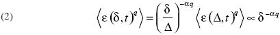
All the dependence on l of the order–q moment is concentrated in the power law δ ^–aq , that is similar to what experimental measures show, namely:

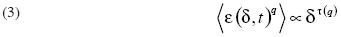
a property which is known as self–similarity. Unfortunately, the exponents obtained in the experiments have not a linear dependence on q in opposition to the usual linear scaling. To describe this "anomalous scaling" Kolmogorov's decomposition can still be applied but now η_δΔ in equation (1) has to be interpreted as a random variable, independent of Δ. The property of self–similarity led researchers to propose a model for its generation based on the existence of local scale–invariant laws.

First, it is assumed that at any point t the following equation holds:

That is, all the dependency on the scale parameter δ is conveyed by the power law factor δ^αt . The exponent α_t , which is a function of the point t under study, is called the singularity exponent of the point. Then, the singularity exponents can be arranged in special sets called singularity components F_α defined as:

In order to close the model, it is required that the singularity components are of fractal character. The singularity spectrum associated to the multifractal hierarchy of fractal components is the function defined by the Hausdorff dimension dim_H of each component F_α, namely

Following Parisi and Frisch (1985) it is possible to derive a relation between self–similarity exponents and the singularity spectrum . They proved that the self–similar exponents could be computed from the Legendre transform of the singularity spectrum ,

By means of equation (7) it is evident that the singularity spectrum contains all the information about self–similarity, that is, it describes the statistics of changes in scale.

The basic hypothesis of this document is that MERVAL, IBOVESPA and IGBVL returns signals are multifractal, meaning that multi–scaling of returns helps to describe real data in a better way than a regular monofractal. This means that the sequence describes the scaling behavior of return absolute moments

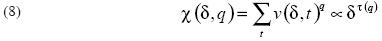
In the same sense as equation (3), and with

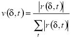
Being the normalized version of returns r(δ, t)= lnP(δ,t + l)– lnP(δ,t) over a time horizon or distance δ , and q the return moment.

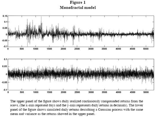
An intuitive interpretation of multifractals in time series analysis consists in thinking of them as a generalization of monofractal models, such as the well–known ordinary Brownian motion, with the difference that in the former case heterogeneity behavior across time is allowed. This, of course, has the advantage of avoiding unrealistic long memory assumptions of monofractals and shows a well characterization of fat tail behavior. Figure 1 shows a comparison between returns modeled from an ordinary Brownian motion and the realization of returns in the New York Stock Exchange (nyse).

 

Methodology

In this section technical analysis for a moving average based crisis–switching indicator of multifractal analysis is exposed.

Crisis–Switching Indicator (CSI)

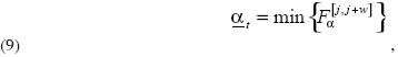
One alternative to analyze the variation of the former multifractal characterization consists in estimating the singularity spectrum performing a rolling window in a time interval [t₀ , t₁ ]. In this sense, one would obtain a series of  sets computed in subintervals: 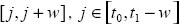. The minimum value for each set can be computed as:

Considering a rolling window [j, j + w] such that there is a unique α_t for each time t and a trajectory α that is constructed only from minimum values, a smooth version of the previous α is achieved by means of a moving average estimator . This leads to an error function of:

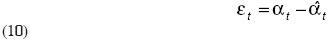
Which is bounded by confidence bands defined as the local maximum (upper bound ξ ^u_t) and local minimum (lower bound ξ ^l_t) of previous errors, defining a set of crossing times constructed by the union 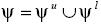with

Where ψ recovers all periods that cross the bands.

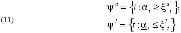
Now let ψ (m) be the m–th element of ψ , and M be the number of crossing times. Then crossing lines are defined as the set of pairs

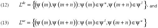
With 0 < m < M; m + n < M such that each element in the first set (L^dc) is called a down–crossing line if n = 1, and a pendular movement of a down crossing line if n > 1. A similar reasoning applies for the second set (L^uc), where each element is an up–crossing line if n = 1, and a pendular movement of an up crossing line if n > 1. Figure 2 shows an example of how crossing lines may actually look like.

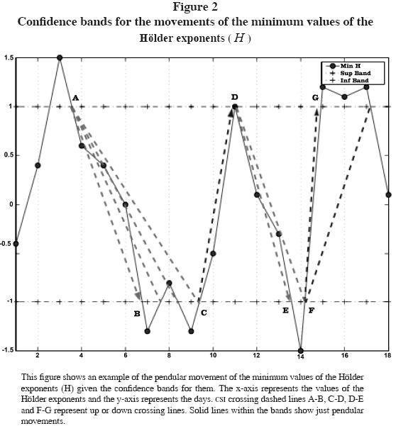
Under a turbulence anticipation context crossing lines and pendular movements are used as crisis–switching indicators for the coming of a crisis. However it is important to mention that the time delay from this point to the development of the crisis may be a rather tricky issue to anticipate. This and other estimation facts will be discussed in the next section.

 

Empirical results

In this section, local multifractal analysis (LMA) and the crisis switching indicator (CSI) based on it are tested for the stock markets indexes of three Latin American emerging markets: MERVAL (Argentina), IBOVESPA (Brazil) and IGBVL (Peru). Table 1 shows the data considered for each case divided in two periods.

For each one of the three indexes 2600 data points were used. The pre–crisis period took the first 1100 observations, while the crisis period used the next 1500 ones. Log versions of time series and its returns were studied for the crisis period. Typical behavior of financial time series such as volatility clustering and fat tails of return's distribution was found for all three series (see figures 3, 4 and 5). Some properties that are harder to analyze, such as log normal volatility, absence of returns correlations, and scale variant distribution of returns, were also verified by basic statistics.

Due to the lack of homogeneous time intervals, the Mexican crisis is manifested at different data points according to the selected time series. Table 2 summarizes the most important dates and data points for all indexes.

It shows two periods for the contagious beginning, one for MERVAL and IBOVESPA (12/21/04), and other for IGBVL (01/09/95), but clearly one highest peak time in 01/10/95. That is a one day reaction delay for the contagious of Argentinean and Brazilian markets, and a reaction of the Peruvian one almost conditioned to the first two crashes.

Multifractal local analysis of stock markets

Singularity spectrums (se) are plotted considering all observations for the three indexes in figure 6 [Chhabra et. al. (1989), and Sornette and Zhou (2006)]. A first inspection reveals that MERVAL and IBOVESPA systems may have similar behavior, with a little more frequency of small anomalies in the latter case showed by the right tail of its parable. On the other hand, the IGBVL case seems to have much more entropy signs through smaller and bigger anomalies, which are probably caused by its pre–crisis period of rather chaotic economic management when compared with the other two indexes.

Local multifractal analysis (LMA) was made by studying changes over time of local singularity spectrums (LSE) for a given time interval. LSE are computed in all indexes for the crisis period using rolling windows of size 1100, so the first computation in the crisis period is done using all the observations of the pre–crisis period (not reported). The potential changes of LSE were assessed by plotting them in the pre–crisis period and in the complete data set (not reported). These computations suggested a clockwise motion in the three cases when the crisis period was added. So, apparently, when a crisis takes effect small anomalies are far more important relative to the big anomalies for the process. This means that negative moments (q) in equation (11) are becoming more important than positive ones, so while the right tail of the parable gets longer, the left one gets shorter (see figure 6).

Patterns around stock market crashes

In order to establish some homogenous pattern around stock market crashes, five basic indicators concerning Hölder exponents were collected from each LSE in the crisis period: minimum, maximum, mean, mode, standard deviation and the one corresponding to the information dimension. These calculations are managed in the usual way in all cases except for the mean and standard deviation indicators. Following Los and Yalamova (2004), in both cases a normalized version is computed by weighting the Hölder exponents (H) by their fractal dimension ( f(H) ).

Figures 7, 8, 9, 10, 11 and 12 show trajectories for some of the indicators mentioned above, letting one suspect of a jump pattern in the minimum series accompanied by an incremental erratic behavior of the maximum series. This finding verifies the adequacy of the crisis–switching indicator (CSI) selected, which basically detects sudden changes in the minimum path (H).

The crisis–switching indicator (CSI) explained before is tested for the three indexes in figures 13, 14, and 15. In all cases moving average estimations and bands construction were made considering parameters t₁ = 1 and t₀ = t – 100 for the crisis period only. CSI empirical results show that it only activates for up crossing lines.

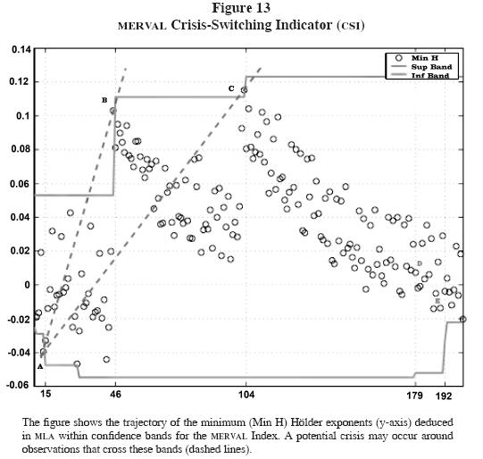
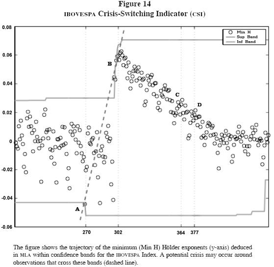
As mentioned in the previous section, even though there is a crossing line pattern before turbulence periods, it is rather difficult to establish a common time delay between the crossing day (the day were the CSI is activated), and the crisis or the climax days. Table 3 summarizes some results concerning CSI estimations.

So it seems that for the Mexican crisis of 12/20/94, one could actually anticipate the stock market crashes in Argentina (MERVAL), Brazil (IBOVESPA) and Peru (IGBVL); in the first two cases about three months before it happened, and for the latter just a few days in advance. Of course, this leads to a very important question about the optimal waiting time for a crisis to happen after the CSI is activated, with a not clear–cut answer. The empirical test of the CSI through a more extend period where dragon and vodka effects are taken into account suggest that the maximum waiting time one should consider is 95 data points, that is, between three and four months.

 

Concluding remarks

It has been showed that patterns in the so–called multifractal path of the minimum Hölder exponents (H) existed around the Mexican crisis of 1994 in the Argentinean (MERVAL), Brazilian (IBOVESPA), and Peruvian (IGBVL) markets. It has also been showed that such patterns are expressed under the form of sudden changes in the H trajectory, and that such changes can be captured in a formal way by means of a crisis–switching indicator (CSI) with about 60 days (observations) in advance. This could be an interesting alert system for monitoring capital markets.

However, there are some issues to clarify before being able to effectively use this tool. For instance, it is not clear why there is not pendular movement in the iboves–pa, when they are present in MERVAL and IGBVL. The same happens for the need of a more profound analysis of the optimal waiting time before a market crash takes effect.

 

References

Agaev, I. and Y. Kuperin (2004). "Multifractal analysis and local Hölder exponents approach to detecting stock markets crashes". Working Paper, Saint–Petersburg State University, Saint–Petersburg.        [ Links ]

Ausloos, M., K. Ivanova and N. Vandewalle (2001). "Crashes: symptoms, diagnoses and remedies". In Empirical Science of Financial Fluctuations, T. Mizuno, M. Katori, H. Takayasu and M. Takayasu eds., Tokyo: Springer.        [ Links ]

Brachet, M., E. Taflin and J. Tcheou (1999). "Scaling transformation and probability distributions for financial time series". EconWPA Paper, No 9901003.        [ Links ]

Chhabra, A., Ch. Meneveau, R. Jensen and K. Sreenivasan (1989). "Direct determination of the ƒ(α) singularity spectrum and its application to fully developed turbulence". Physical Review Online Archive, 40(9), 5284–5294.        [ Links ]

Kolmogorov A. (1941a). "Dissipation of energy in the locally isotropic turbulence". Dokl. Akad. Nauk SSSR, 32, 16–18.        [ Links ]

––––––––––(1941b). "The local structure of turbulence in incompressible viscous fluid for very large Reynolds numbers". Proceedings: Mathematical and Physical Sciences, 34(1890), 9–13.        [ Links ]

Los, C. and R. Yalamova (2004). "Multi–fractal spectral analysis of the 1987 stock market crash". EconWPA Paper No 0409050.        [ Links ]

Lovejoy, S., D. Schertzer and F. Schmitt (2002). "Multifractal fluctuations in finance". International Journal of Theoretical and Applied Finance, 3(3). 361–364.        [ Links ]

Mandelbrot, B. (1967). "How long is the coast of Britain? Statistical self–similarity and fractional dimension". Science, 156(3775), 636–638.        [ Links ]

––––––––––(1972). "Possible Refinement of Lognormal hypothesis concerning the distribution of energy dissipation in intermittent turbulence". Statistical Models and Turbulence, M. Rosenblatt and C. Van Atta eds., Lecture Notes in Physics 12, Springer–Verlag, New York, 333–351.        [ Links ]

––––––––––(1975). "Geometry of homogeneous scalar turbulence: iso–surface fractal dimensions 5/2 and 8/3". Journal of Fluid Mechanics, 72(2), 401–416.        [ Links ]

––––––––––(1997). "Fractals and Scaling in Finance: Discontinuity, Concentration and Risk". Netherlands: Springer–Verlag.        [ Links ]

Muzy, J., J. Delour and E. Bacry (2000). "Modelling fluctuations of financial time series: from cascade process to stochastic volatility model euro". Physics Journal B 17, 537–548        [ Links ]

Parisi, G. and U. Frisch (1985). "On the singularity structure of fully developed turbulence". Turbulence and Predictability in Geophysical Fluid Dynamics and Climate Dynamics, M. Ghil (ed.). North–Holland.        [ Links ]

Sornette, D. and W. Zhou (2006). "Importance of positive feedbacks and overconfidence in a self–fulfilling using model of financial markets". Physica A: Statistical Mechanics and its Applications, 370(2), 704–726.        [ Links ]