


 texto em
  Inglês (pdf)
 Artigo em XML
 Referências do artigo
 Enviar este artigo por email
 Citado por SciELO
  Similares em
SciELO
Similares em
SciELO 
 Permalink
Introduction
The Gulf of California (GC) is a highly biodiverse marginal sea with high primary productivity comparable to that of the Bay of Bengal, North Africa, and the California Current (Álvarez-Borrego and Lara-Lara 1991). However, most studies on the composition, diversity, and productivity of phytoplankton in the GC have focused on the coastal zone, which is rich in nutrients due to upwelling events and tidal mixing (e.g., Maciel-Baltazar and Hernández-Becerril 2013). In contrast, notwithstanding that the deep and remote regions in this sea have less productive conditions, studies on these zones are relatively scarce. The Guaymas Basin (GB) stands out as an example of this; in this region, high surface temperatures occur during the summer and they produce strong vertical stratification, which impedes or significantly decreases the flux of nutrients from subsurface waters (Segovia-Zavala et al. 2010, White et al. 2013). This flux produces oligotrophic conditions, which could limit or promote changes in the composition, diversity, and productivity of phytoplankton. Thus, it is extremely important to identify the mechanisms and factors involved in fertilization processes in this area. In this respect, previous studies have reported the prominent role played by diazotrophic cyanobacteria blooms in the GC region, as these bacteria are important nitrogen (N) fixers that significantly support primary productivity in this basin (White et al. 2007, 2013). In this context, the aim of the current study is to assess the taxonomic composition of phytoplankton to identify the factors that determine their behavior in oligotrophic surface waters in the central region of the GC.
Materials and methods
Study area
The GC is located between 23° and 32° N and 108° and 115° W. It has a NW to SE orientation, measures approximately 1,100 km long and 150 km wide, and communicates with the Pacific Ocean on its southern part. In the GC, the surface layer has a thermohaline circulation that depends on seasonal physical processes; on the other hand, subsurface waters associated with the oxygen-minimum layer, which extends from the NE of the tropical Pacific to the central region of the GC, influence some chemical properties (dissolved oxygen, pH, and nutrients) (Delgadillo-Hinojosa et al. 2006). In general, there are 2 distinctive seasons in the GC during the seasonal cycle: the cold season and the warm season. The cold season extends from December to May and is characterized by low surface temperatures and a deep mixed layer, especially in February, as a result of forcing by prevailing winds and thermal convection (Robles and Marinone 1987). By contrast, in the warm season, between June and October, surface temperature increases and the water column stratifies (Valdez-Holguín et al. 1999). During this period, supply of nutrients from deep waters is limited and the surface layer above the nutricline is remarkably depleted in nitrates (White et al. 2007, Torres-Delgado et al. 2013).
Sample collection
From 3 to 5, September 2016, the EXFINIFE cruise was carried out aboard the research vessel Alpha Helix in the central region of the GC. During these 3 days, 4 samplings were done at a point located in GB (27°12ʹ N, 111°18ʹ W) (Fig. 1a): 3 September, D1; 4 September, D2; and 5 September, D3-1 and D3-2. Samplings were done in late summer during neap tide conditions. These conditions favor the presence of phytoplankton groups typical of oligotrophic conditions (White et al. 2007, Segovia-Zavala et al. 2010).

Figure 1 Location of the sampling station ( ). Satellite image of chlorophyll a (Modis-Aqua, 8-day composite: 28 August to 4 September 2016) (a) and spatiotemporal distribution of temperature (b), salinity (c), sigma-t (d), and fluorescence (e). For the elaboration of the cross sections for temperature, density, salinity, and fluorescence, a linear interpolation scheme was used in the Ocean Data View program.
Hydrographic casts were carried out using a CTD (SeaBird Electronics, model SBE 9-11 plus) equipped with conductivity, temperature, dissolved oxygen, and fluorescence sensors, during daylight hours: 5 casts in D1, 6 casts in D2, and 4 casts in D3-1 and D3-2. The depth at the sampling point is ~2,000 m; however, to analyze chlorophyll a (Chla), phytoplankton, dissolved iron (Fed), nitrates plus nitrites (NO3 + NO2), phosphates (PO4), and silicates (SiO4), water samples were collected at 3 different depths, equal to or less than 50 m (5 m, 25-35 m, and 37-50 m), using 5-L Niskin bottles (General Oceanics) coupled to a rosette. Sampling depths were chosen according to the potential of photosynthetic activity corresponding to the surface (5 m), ~50% of surface irradiance (I0), and the fluorescence maximum (7‒9% of I0). To analyze Chla, 1 L of seawater was filtered through glass fiber filters (GF/F, 25 mm). After the water was filtered, filters were placed in HistoPrep capsules, which were stored in liquid nitrogen until their analysis in the laboratory. To analyze Fed, water was collected under ultra-clean conditions (Bruland et al. 2001, Delgadillo-Hinojosa et al. 2006, Segovia-Zavala et al. 2010). Water samples for abundance estimation and phytoplankton identification were preserved in acidified Lugol’s solution at 1% final concentration and stored in the dark at 4 °C. To analyze nutrients, water was kept in 20-mL dark plastic bottles at -20 °C until analysis in the laboratory.
Analysis of variables
Dissolved iron and inorganic nutrients
The Fed was pre-concentrated using the organic extraction method with the ammonium 1-pyrrodyldithiocarbamate/diethylammonium diethyldithiocarbamate (APDC/DDDC) chelator (Bruland et al. 2001, Segovia-Zavala et al. 2010), and a back-extraction step was added (Félix-Bermúdez et al. 2020). Fed concentration was determined by graphite furnace atomic absorption using an Agilent 280Z AA spectrophotometer equipped with Zeeman background correction. Analyses of inorganic nutrients (NO3 + NO2, PO4, and SiO4) in the dissolved fraction were done using colorimetric techniques (Gordon et al. 1993) with an AA3 Skalar SANPlus continuous segmented flow autoanalyzer (Seal Analytical, United Kingdom).
In situ chlorophyll a and satellite chlorophyll
Prior to analysis, filters for Chla determination were thawed, immediately placed in 10 mL of 90% acetone for 24 h, and kept in the dark at 4 °C. Chla concentration was determined using an Agilent Technologies Cary 50 UV-Visible spectrophotometer and the equation by Jeffrey and Humphrey (1975). The satellite chlorophyll (Chlsat) image, derived from the MODIS-Aqua sensor, was an 8-day composite (28 August to 4 September, 2016) with level 3 and spatial resolution of 4 × 4 km. Image processing was performed using the SeaDAS 7.3.2 program (https://oceancolor.gsfc.nasa.gov, accessed 3 April 2021).
Nano-microphytoplankton and diazotrophic cyanobacteria
For the phytoplankton analysis, cells were counted and measured according to Hasle (1978). The technique consists in concentrating 100 mL of seawater in a sedimentation chamber for a 48-h period. Phytoplanktons were mostly classified at the highest taxonomic level using the techniques used by Gómez (2013). Diatoms and diazotrophic cyanobacteria were measured with a micrometer adapted to a Zeiss Axio Vert.A1 microscope. Subsequently, diatom measurements were transformed to biovolume (µm3) using the stereometric forms suggested by Strathmann (1967) and Edler (1979). Diatom biomass was determined by size fraction: nanodiatoms (5-20 µm) and microdiatoms (>20 µm). The abundance of Trichodesmium spp. and Richelia sp. was determined in cells per liter. The following equation was used to calculate diatom and picophytoplankton biomass:
where B p is the biomass of the cell population (μg C·L-1), C p is the abundance of organisms (cell·L-1), V p is the cell biovolume (μm3 cell·L-1), and F p is the biovolume to carbon conversion factor using the equation pg C·cell-1 = 0.443 × (µm3)0.863 (Verity et al. 1992).
Picophytoplankton
For the picophytoplankton analysis, seawater samples were fixed in formaldehyde, which was neutralized with sodium borate to a final concentration of 1%, and stored at -4 °C under dark conditions (this fixative may cause count underestimation). Subsequently, in the laboratory, they were filtered with a 0.2-μm polycarbonate membrane and mounted on slides with low-fluorescence immersion oil for epifluorescence counting (MacIsaac and Stockner 1993). Cells with circular and ovoid morphology and red-orange autofluorescence were counted at 1,200× magnification with excitation light of blue wavelength (450-490 nm).
Results
Hydrographic conditions
During 3 days of sampling, the water column changed from strongly stratified to partially mixed. The depth of the 22 kg·m-3 isopycnal was approximately 30 m during the first 2 days of sampling (D1 and D2) (Fig. 1d). This was caused by higher average values of salinity (35.41 ± 0.06) and temperature (30.69 ± 0.11 °C) recorded in the layer above 30 m (hereinafter called the surface layer) than average values of salinity (35.23 ± 0.10) and temperature (24.82 ± 2.91 °C) recorded below 30 m (hereinafter called the deep layer). Nonetheless, a decrease in salinity and average temperature in the surface layer (35.34 ± 0.05 and 28.30 ± 1.60 °C) during the third day of sampling (D3-1 and D3-2) resulted in an abrupt uplift of the 22 kg·m-3 isopycnal, which indicated a change from stability to relative instability in the water column (Fig. 1d).
Biogeochemical variables
Chemical variables
Inorganic nutrients behaved similarly during the 3 days of sampling, with low concentrations in the surface layer and high concentrations in the deep layer (Fig. 2a-c). Averages found for NO3 + NO2, PO4, and SiO4 were, respectively, 0.02 ± 0.00, 0.58 ± 0.17, and 3.49 ± 1.12 µM in the surface layer and 2.29 ± 2.08, 0.95 ± 0.22, and 8.16 ± 3.44 µM in the deep layer (Table 1). On the first day of sampling (D1), the vertical distribution of Fed showed lower mean concentrations in the surface layer and higher in the deep layer (2.50 ± 0.00 nM and 4.60 ± 2.40 nM, respectively; Fig. 2d). In contrast, means for samplings of the second (D2) and third (D3) days had very similar values for the surface layer and the deep layer (1.19 ± 0.46 and 1.29 ± 0.22 nM, respectively; Table 1).

Figure 2 Vertical distribution of nitrates plus nitrites (NO3 + NO2) (a), phosphates (PO4) (b), silicates (SiO4) (c), and dissolved iron (Fed) (d) in the samples from the Guaymas Basin during the late summer of 2016.
Table 1 Physicochemical and biological variables measured during the EXFINIFE cruise carried out in the Guaymas Basin from 3 to 5 September 2016. Depth (Z, m); temperature (T, °C); salinity (S); chlorophyll a (Chla, mg·m-3); diatoms (Diato., cell·L-1); dinoflagellates (Dino., cell·L-1); Trichodesmium spp. (Trich., cell·L-1); Richelia sp. (Rich., cell·L-1); picophytoplankton (Pico., cell × 106·L-1); nano-microdiatom biomass (BND-BMD, µg C·L-1); picophytoplankton biomass (BPico., µg C·L-1); irradiance (I0, %); nitrates plus nitrites (NO3 + NO2), phosphates (PO4), and silicates (SiO4) (detection limit of 0.02, 0.02, and 0.04 µM, respectively); and dissolved iron (Fed, 0.04 nM detection limit).
| Survey | Z | T | S | Chla | Diato. | Dino. | Trich. | Rich. | Pico. | BND-BMD | BPico. | I0 | NO3 + NO2 | SiO4 | PO4 | Fed |
| D1 | 5 | 30.61 | 35.37 | 0.33 | 1,717 | 8,623 | 1,043 | 28.8 | 1.39-3.42 | 32.70 | 100 | 0.02 | 3.08 | 0.51 | 2.47 | |
| 35 | 28.94 | 35.25 | 0.32 | 1,770 | 5,379 | 3,128 | 33.8 | 0.54-89.30 | 37.40 | 15 | 0.02 | 3.67 | 0.80 | 2.86 | ||
| 50 | 22.20 | 35.09 | 0.39 | 10,872 | 5,050 | 5,214 | 18.3 | 42.90-122.60 | 20.70 | 5 | 3.80 | 9.24 | 6.31 | |||
| D2 | 5 | 30.77 | 35.46 | 0.48 | 677 | 6,088 | 2,085 | 23.3 | 0.12-5.25 | 26.41 | 100 | 0.02 | 2.24 | 0.38 | 1.63 | |
| 35 | 24.57 | 35.22 | 0.78 | 31,285 | 11,411 | 1,564 | 49.7 | 71.73-1,590.00 | 56.30 | 15 | 0.06 | 6.03 | 0.84 | 1.53 | ||
| 45 | 23.59 | 35.35 | 0.80 | 17,747 | 11,091 | 417 | 21.6 | 20.41-422.30 | 24.50 | 5 | 3.24 | 9.14 | 1.24 | |||
| D3-1 | 5 | 29.08 | 35.36 | 0.33 | 1,408 | 4,629 | 2,086 | 28.1 | 1.00-4.96 | 31.90 | 100 | 0.02 | 3.75 | 0.65 | 0.71 | |
| 25 | 26.45 | 35.29 | 0.61 | 4,218 | 6,190 | 134.0 | 3.70-105.19 | 151.90 | 20 | 0.02 | 4.89 | 0.77 | 1.24 | |||
| 40 | 24.45 | 35.29 | 0.94 | 8,861 | 4,421 | 89.7 | 14.94-1,828.00 | 101.70 | 10 | 4.31 | 12.70 | 1.20 | 1.10 | |||
| D3-2 | 5 | 29.23 | 35.38 | 0.19 | 989 | 5,261 | 31.1 | 0.59-5.01 | 35.30 | 100 | ||||||
| 33 | 25.59 | 35.34 | 0.74 | 5,269 | 4,612 | 147.0 | 6.18-230.24 | 166.60 | 20 | |||||||
| 37 | 25.06 | 35.35 | 1.02 | 8,729 | 4,878 | 64.9 | 11.07-293.90 | 72.40 | 10 |
Taxonomic composition of phytoplankton (>5 µm)
Diatom richness (>5 µm) consisted of 42 taxa in total, of which 7 belonged to Chaetoceros, 6 to Rhizosolenia, 3 to Coscinodiscus, 2 to Guinardia, 2 to Actinoptychus, and 2 to Bacteriastrum (Table 2). Likewise, 20 genera were identified, each with a morphospecies. Dinoflagellates (not included in Table 2) showed 26 taxa, distributed in 7 Tripos species (Tripos fusus, Tripos furca, Tripos azoricus, Tripos macroceros, Tripos candelabrus, Tripos lineatum, and 1 Tripos sp.), 3 Gymnodinium (Gymnodinium catenatum and 2 Gymnodinium spp.), 2 Gyrodinium (Gyrodinium spirale and 1 Gyrodinium sp.), 3 Oxytoxum (Oxytoxum laticeps, Oxytoxum sceptrum, and Oxytoxum scolopax), 2 Prorocentrum (Prorocentrum gracile and Prorocentrum micans), 2 Protoperidinium (Protoperidinium corniculum and Protoperidinium acutum), Scrippsiella trochoidea,Podolampas palmipes, Gonyaulax polygramma, Ornithocercus magnificus, Amphisolenia bidentata, Brachidinium capitatum, and Peridinium sp.
Table 2 List of marine phytoplankton diatoms (Bacillariophyta) identified during the EXFINIFE cruise carried out in the Guaymas Basin from 3 to 5 September 2016. The symbols indicate the size (<20 µm, >20 µm) of the taxon determined from the volume of the sphere.
| Survey/depth | ||||||||||||
| D1 | D1 | D1 | D2 | D2 | D2 | D3-1 | D3-1 | D3-1 | D3-2 | D3-2 | D3-2 | |
| Nano-microdiatoms | 5 m | 35 m | 50 m | 5 m | 35 m | 45 m | 5 m | 25 m | 40 m | 5 m | 33 m | 37 m |
| Cylindrotheca closterium (Ehrenberg) | < | < | < | < | < | < | < | < | < | < | < | < |
| Nitzschia longissima (Kützing) | < | < | < | |||||||||
| Pseudo-nitzschia seriata (Cleve) | < | < | < | < | < | < | < | < | ||||
| Rhizosolenia longissima (Grunow) | > | > | > | > | > | > | < | < | > | > | > | < |
| Rhizosolenia clevei (Ostenfeld) | > | > | > | > | > | > | > | |||||
| Rhizosolenia bergonii (Peragallo) | > | > | > | > | > | |||||||
| Rhizosolenia imbricata (Brightwell) | > | > | > | |||||||||
| Rhizosolenia acuminata (Peragallo) | > | |||||||||||
| Rhizosolenia setigera (Brightw) | < | > | > | < | < | < | > | |||||
| Pseudosolenia calcar-avis (Schultze) | > | > | ||||||||||
| Proboscia alata (Brightwell) | > | > | > | > | > | |||||||
| Coscinodiscus radiatus (Ehrenberg) | > | > | > | > | > | > | > | > | > | |||
| Coscinodiscus gigas (Ehrenberg) | > | > | > | > | > | > | > | |||||
| Coscinodiscus curvatulus (Grunow) | > | > | > | > | < | < | < | < | ||||
| Leptocylindrus danicus (Cleve) | < | < | < | < | < | < | < | < | ||||
| Chaetoceros affinis (Gran) | < | < | ||||||||||
| Chaetoceros messanensis (Castracane) | < | < | < | < | < | < | < | < | < | < | ||
| Chaetoceros lorenzianus (Grunow) | > | > | > | |||||||||
| Chaetoceros radicans (Schütt) | < | < | < | < | < | < | < | < | < | |||
| Chaetoceros pseudoaurivilli (Ikari) | > | |||||||||||
| Chaetoceros peruvianus (Brightwell) | > | > | ||||||||||
| Chaetoceros curvisetus (Cleve) | < | < | < | |||||||||
| Guinardia delicatula (Cleve) | > | > | > | |||||||||
| Guinardia striata (Stolterfoth) | > | > | > | > | > | > | > | > | ||||
| Actinoptychus splendens (Shadbolt) | > | > | > | |||||||||
| Actinoptychus senarius (Ehrenberg) | > | > | > | > | ||||||||
| Bacteriastrum elegans (Pavillard) | > | |||||||||||
| Bacteriastrum delicatulum (Cleve) | < | < | ||||||||||
Of the trichome-forming diazotrophic cyanobacteria, 2 species of Trichodesmium (Trichodesmium erythraeum Ehrenberg ex Gomont, 1892 and Trichodesmium sp.) and one symbiotic species (Richelia intracellularis J. Schmidt, 1901) associated with diatoms of the genus Rhizosolenia were detected. Within the group of silicoflagellates, Distephanus speculum, Dictyocha fibula, and one unidentified morphospecies in the group of coccolithophores were identified. Other abundant phytoplankton individuals, with unidentified cells <13 µm, were grouped into the phytoflagellate category considering their morphology.
Biomass and abundance of phytoplankton
Figure 3 shows the vertical profiles of Chla concentrations and the biomass as quantified from 2 groups of phytoplankton (diatoms plus autotrophic picophytoplankton). Although considerable temporal variability of Chla and phytoplankton biomass was observed, both variables were closely correlated (Spearman’s r = 0.75, n = 12, P < 0.05). With the exception of the Chla profile for sampling D1, where there was little vertical variability, the maximum values of Chla and biomass were observed in the subsurface (Fig. 3a-b). Overall, average surface biomass, characterized by contributions of autotrophic picophytoplankton, nanodiatoms, and microdiatoms (~85.0%, 2.0%, and 13.0%, respectively), was ~20 times lower than that in the deep layer (10.0%, 8.0%, and 82.0%, respectively). In particular, biomass maxima in D2 (1,718 µg C·L-1) and D3-1 (1,944 µg C·L-1) were 4 times higher than in D3-2 (403 µg C·L-1).

Figure 3 Vertical profiles of chlorophyll a concentration and biomass of phytoplankton groups (diatoms plus autotrophic picophytoplankton) in samples collected during the 3 days of sampling (D1, D2, D3-1, and D3-2) in the Guaymas Basin during the late summer of 2016.
Phytoplankton (>5 µm) had higher abundances in D2 than in the other samplings, with a maximum of 60 × 103 cell·L-1 at 35 m (Fig. 4). Meanwhile, picophytoplankton (<2 µm) showed subsurface maxima, although of lesser magnitude in D1 and D2 than in D3-1 and D3-2 (134 and 147 × 106 cell·L-1, respectively) (Fig. 4). Regarding the contribution of phytoplanktonic groups to the abundance of the >5 µm fraction, indeterminate phytoflagellates and dinoflagellates predominated in surface samples (average: 44.0% and 39.0%, respectively); conversely, diatoms predominated in samples from the deepest stratum (43.0%). In the intermediate stratum, the average contribution was similar between the 3 groups (30.0-32.0%). The records of trichome-forming diazotrophic cyanobacteria were, in general, very irregular, and relatively low abundances were recorded (between undetectable and 5.21 × 10³ cell·L-1), with Trichodesmium spp. being observed mainly in D1 and D2 at 5 m. In contrast, Richelia intracellularis was not detected in D1, but it was found in D2 at 35 and 45 m and in D3-1 at 5 m (Table 1). These diazotrophs and other phytoplanktonic groups (coccolithophores and silicoflagellates) contributed, respectively, up to 22.0% (e.g., in D1 at 35 m) and 1.2% (e.g., in D2 at 35 m) of the abundance of the >5 μm fraction (Fig. 4).
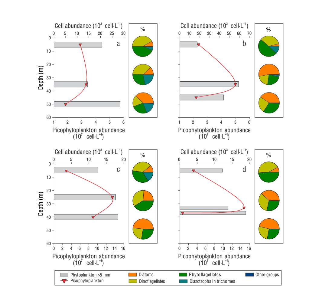
Figure 4 Vertical profiles of the total abundance of phytoplankton >5 μm and diagrams of the relative contribution of the main phytoplankton groups (%) to the abundance of samples collected in the Guaymas Basin during the late summer of 2016: September 3, D1 (a); September 4, D2 (b); and September 5, D3-1 (c) and D3-2 (d).
Discussion
Hydrography
In the study area, vertical stability was well-defined in D1 and D2 (Fig. 1b, c). However, in D3-1 and D3-2, temperature and salinity decreased in the surface layer. The change from vertical stability to a partial mixture observed during samplings D3-1 and D3-2 could be related to the increase in wind speed and wave height experienced in the region with the influence of Hurricane Newton (https://www.nhc.noaa.gov/archive/2016/ep15/ep152016.publica.005.shtml?, accessed October 2016), which, in addition to limiting the continuity of the study, decreased the euphotic area by 10 m (70 to 60 m) and the depth of the mixed layer by 50% (30 to 15 m).
Spatial and temporal variability of nutrients
Despite partial weakening of the vertical stratification in D3-1 and D3-2, oligotrophic conditions were observed throughout the study. Average ratios of N:P (0.55 ± 1.34), N:Si (0.13 ± 0.18), and Fe:N (52.70 ± 29.70) indicated that the limiting nutrient during this study was N. The main supply of N to the surface layer in the central region of the GC comes from the deeper layers and is modulated by processes of convection, advection, and diapycnal and/or turbulent diffusion (Lavín et al. 1995, Torres-Delgado et al. 2013). However, the waters of these deeper layers tend to be deficient in the content of N (N:P < 16) available to non-diazotrophic primary producers (Dutkiewicz et al. 2012, Torres-Delgado et al. 2013). This occurs because the water masses they belong to underwent denitrification processes in the oxygen minimum zone of the tropical northeastern Pacific (Delgadillo-Hinojosa et al. 2006), which reduces the usable N content for non-diazotrophic primary producers (Dutkiewicz et al. 2012).
Phytoplankton structure
The phytoplankton composition was representative of transition zones, with species from both coastal and oceanic conditions, and is characterized by an important contribution of diatoms, dinoflagellates, and phytoflagellates. Comparable to our results, Hernández-Becerril (1987) reported a richness of 60 species and 3 unidentified morphotypes in the central region of GC during June 1982, with a contribution of diatoms and dinoflagellates of 48.0% and 33.0%, respectively, in relation to total phytoplankton taxa >5 μm.
The high contribution of some dinoflagellate species (e.g., Tripos fusus, Tripos furca, Tripos macroceros, Tripos candelabrus, Prorocentrum gracile, Prorocentrum micans, Oxytoxum sceptrum, and Oxytoxum scolopax) to phytoplankton >5 μm in the surface layer was characterized by the presence of species that show high motility, the capacity to regulate their position in the water column, and slower growth to conserve biomass and manage resources in oligotrophic and high irradiance conditions (Reynolds 1991). At intermediate depths, we detected an important component of centric nanodiatoms (e.g., Chaetoceros messanensis, Chaetoceros radicans, Chaetoceros curveetus, Leptocylindrus danicus) and dinoflagellates (e.g., S. trochoidea, Oxytoxum laticeps), characterized by a high surface-to-volume ratio. This high ratio allows them to assimilate nutrients rapidly and achieve high growth rates in environments with low levels of disturbance (Reynolds et al. 2002). Under oligomesotrophic conditions of the thermocline, we observed the coexistence of diatoms with strategies similar to those of diatoms in the intermediate level and populations of diatoms of larger size and morphology (e.g., Rhizosolenia clevei, Rhizosolenia bergonii, Rhizosolenia imbricata, Coscinodiscus gigas, Coscinodiscus radiatus, and Actinoptychus senarius), with high uptake and nutrient requirements (Reynolds 1991).
Phytoplankton biomass
The results indicate that diatoms tended to accumulate in deeper levels and showed a vertical distribution similar to that of fluorescence (Figs. 1e, 4). This accumulation of diatoms occurs because the deepest waters contain the highest concentrations of nutrients, mainly NO3 + NO2, and because diatoms are ecophysiologically adapted with photoacclimation capacities, as Chla per cell increases with depth (Latasa et al. 2017). In contrast, other relatively abundant groups in the surface layer, composed of dinoflagellate species and picophytoplankton ecotypes, are characterized by greater affinities to oligotrophic conditions (e.g., those with heterotrophic or mixotrophic capacity) and adaptations to high irradiances (e.g., low chlorophyll b 2/a 2 ratios and variations in their phycoerythrin content) (Ong and Glazer 1991, Moore and Chisholm 1999) (Fig. 4).
The temporal resolution of the fluorescence profiles, as an indicator of phytoplankton biomass, confirms the association of phytoplankton dynamics with photoadaptation to light intensity combined with availability of inorganic nutrients (Fig. 1e). This distribution shows a predominantly oligotrophic layer in the first few meters, and a subsurface maximum between ~40 and 55 m that tends to deepen slightly and increase in magnitude during the afternoon hydrographic casts (Figs. 1e, 4c). The latter is reflected by the significant correlations (P < 0.05) observed between Chla and depth and temperature (ρ = 0.58 and ρ = -0.61, respectively; n = 12). The subsurface maximum of Chla is a common feature in vertically stratified environments and, in general, coincides with the shallowest part of the nutricline and with optimal irradiance conditions (Cullen 2015). This indicates that low concentrations of Chla detected at surface levels in this study could be a consequence of excessive irradiance (>1,500 µE·m-2·s-1) and low concentrations of NO3 + NO2, which may limit phytoplanktonic growth. On the other hand, in intermediate-to-deep waters, abundance of nutrients and acclimation of phytoplankton to irradiation and its spectral quality stimulate the growth of microphytoplankton cells and, therefore, increase the concentration of photosynthetic pigments and biomass (Klausmeier and Litchman 2001). This increase is observed in the significant correlations (P < 0.05) of Chla with the concentration of NO3 + NO2 (ρ = 0.68, n = 9) and depth (r = 0.58, n = 12). In summary, low concentrations of NO3 + NO2 and excess irradiance at the surface do not favor the proliferation of diatoms, which is in agreement both with the significant correlation between diatoms and Chla (P < 0.05, ρ = 0.68, n = 12) and with the high contribution of Chla to the biomass of nano-microdiatoms. This observation is consistent with the Chlsat values from MODIS-Aqua at the first optical depth (~20 m, Fig. 1a), which were very similar to the Chla concentration of the D1 sampling at 5 and 35 m (Table 1, Fig. 3a).
Low Chla concentrations detected at the surface coincide with a relative increase in picophytoplankton biomass of 85.0% with respect to diatoms. This predominance can be explained by the high surface-to-volume ratio that characterizes very small cells and, consequently, by how efficiently these absorb nutrients compared to larger fractions (Chisholm 1992, Raven et al. 2005). This contribution to biomass is similar to the 75.0% contributed by picophytoplankton (Synechococcus and Prochlorococcus) reported by Miranda-Alvarez et al. (2020) for the surface waters of the northeastern region of the tropical Pacific. Moreover, the association between intervals of Chla and values of the relative contribution to autotrophic biomass of the size fractions observed here is very similar to that reported for the southern region of the California Current (Taylor and Landry 2018).
The above-mentioned association indicates that the supply of nutrients, which depends on the degree of stability in the water column (Karl and Lukas 1996, Falkowski 1997), and the degree of photoadaptation to light intensity controlled the presence and abundance of certain phytoplankton groups in surface waters of the GC.
Spatiotemporal variability of diazotrophic cyanobacteria
The presence of diazotrophic cyanobacteria in this work was very irregular and showed relatively low abundances (2,220 ± 1,575 cell·L-1). These abundances are comparable to the indirect quantifications from Richelia intracellularis trichomes (<40-1,700 trichomes·L-1, assuming a range of 3-5 vegetative cells in symbiosis per trichome), and Trichodesmium spp. nifH genes (0-624 copies of cDNA·L-1) previously performed by White et al. (2007, 2013) in the GB in summer. Trichodesmium spp. was found at all depths in D1 and at 5 m in D2, but was absent in D3-1 and D3-2 (Table 1). Conversely, Richelia intracellularis was not detected in D1, but was found at 35 and 45 m in D2 and 5 m in D3-1 (Table 1). This suggests that, despite favorable conditions of vertical stratification, high temperature, and low concentrations of inorganic N, the proliferation of these organisms could have been limited by factors not evaluated in this study (e.g., concentration of micronutrients, grazing, competition, etc.).

