


 texto en
  Inglés (pdf)
 Artículo en XML
 Referencias del artículo
 Enviar artículo por email
 Citado por SciELO
  Similares en
SciELO
Similares en
SciELO 
 Permalink
INTRODUCTION
Among billfish species (family Istiophoridae), the striped marlin, Kajikia audax (Philippi, 1887), has the widest latitudinal distribution (between 45° N and 45° S) in subtropical and temperate regions (20 to 25° C) from the Indian and Pacific oceans (Howard and Ueyanagi 1965, Squire and Suzuki 1990, Domeier et al. 2003, McDowell and Graves 2008). In the Pacific Ocean, the distribution areas of the striped marlin are configured in the shape of a horseshoe with 2 transoceanic regions in each hemisphere (northern and southern) joined at their eastern end along the coast of the American continent (Squire and Suzuki 1990). The striped marlin is particularly abundant off the coast of the Baja California Peninsula and at the mouth of the Gulf of California, a relevant area that is considered a center of population concentration for striped marlin, both for its exploitation and for its fishery management (Squire 1987). In this region, this species has been exploited for more than 50 years, by commercial fleets and recreational fleets.
Recreational fishing had its origins around 1930, when recreational fishermen from the United States traveled in their own boats to the south of the Baja California Peninsula, between Cabo San Lucas and La Paz. In the 1960s, Cabo San Lucas was still reported as a place with good fishing spots, and the development of hotel services for recreational fishermen began (Talbot and Wares 1975). Currently, the main recreational fleets concentrate at the mouth of the Gulf of California, near the center of highest availability of striped marlin in the eastern Pacific (Ortiz et al. 2003, Domeier 2006), and they depend on the abundance of this species in the region. Despite its long history, recreational fishing in Mexico had its biggest growth in the early 1990s, and, to date, the effect of this fishery on striped marlin abundance has not been evaluated.
Commercial exploitation began in the late 1950s, when tuna fleets from Japan expanded their fishing areas to the eastern Pacific. In 1963 they reached the region off the Baja California Peninsula, where catches of striped marlin were large and equal to those of tuna (Talbot and Wares 1975). In the 1970s, with the declaration of the exclusive economic zone (EEZ) of Mexico, there was a transition to Mexican fleets focused on tuna, shark, and finfish fishing, where striped marlin formed an important part of the bycatch. In 1984, the first specific commercial fishing permits were issued for several billfish species, with striped marlin making up the majority of these catches. In 1991, permits were no longer granted for striped marlin fishing, and the fleets shifted to swordfish fishing. Eventually, many of these vessels turned to shark fishing; therefore, since the 1990s, these fleets have caught striped marlin incidentally. The status of striped marlin in the Pacific coast of Mexico was analyzed by Klett-Traulsen and Aguilar-Ibarra (2001) using the historical series of commercial catches available at that time, that is, from 1963 to 1990, which represents a period of intense fishing by both Japanese and Mexican longline fleets. Klett-Traulsen and Aguilar-Ibarra (2001) did not include recreational fishing in their model, and for the time period covered by the study, bycatch was considered insignificant. Other assessments of striped marlin that have greater geographic coverage in the eastern Pacific Ocean are found in the works of Hinton and Bayliff (2002), Hinton and Maunder (2004), Hinton (2009), and Hinton and Maunder (2009) (Fig. 1a).

Figure 1 Study area. (a) Study area (shaded area) in relation to assessment areas that are managed in other striped marlin assessments (A1-A3) (e.g., Hinton and Maunder 2009). (b) Area of influence (shaded area) of the commercial and tuna fleets. (c) Area of influence (dotted area) of recreational fleets. (d) Area of influence (area with diamond pattern) of billfish and shark fleets. I: Ensenada, Baja California; II: La Paz, Baja California Sur; III: Guaymas, Sonora; IV: Mazatlán, Sinaloa; V: Manzanillo, Colima; and VI: Acapulco, Guerrero.
Currently, the management of striped marlin in Mexico focuses on recreational fishing and the bycatch produced by billfish and shark fisheries. Management guidelines are found in different legal documents (DOF 2007, 2012, 2013) and several current agreements dating back to the 1980s (DOF 1987, 1994, 2008). Given the importance of the species, this work evaluates the state of exploitation of the striped marlin that is distributed off the Pacific coast of Mexico with a historical series of more than 50 years, which includes commercial, recreational, and incidental catches.
MATERIALS AND METHODS
Catch and effort
The catch and effort data used in this study came from commercial and recreational fishing fleets that have operated in the EEZ of Mexico in the Pacific between 1963 and 2014 (Fig. 1b-d). All catches were expressed in number of individuals, whereas effort was quantified in different units, which are detailed in Table 1. The information on commercial fishing directed at striped marlin came from Japanese and Mexican longline fleets (1963-1990), which were considered as a single commercial fleet (f 1) with an index of relative abundance, which was already standardized (Klett-Traulsen and Aguilar-Ibarra 2001). The information on recreational fishing came from 2 sources that covered different periods. The first source was taken from the work of Squire (1987); this contained information from 1969 to 1984, from which data from Baja California were selected: Guaymas, Kino Bay, and Puerto Peñasco (Sonora); Mazatlan (Sinaloa); and Acapulco, Zihuatanejo, and Ixtapa (Guerrero). We handled these data as coming from a single fleet (f 2). The second source covered information from 1985 to 2014, which came from monthly samplings and daily catch reports provided by the recreational fishing fleets of 3 key ports at the mouth of the Gulf of California: Cabo San Lucas, Buenavista, and Mazatlán. This information came from the Programa de Monitoreo de Pesca Deportiva (Sport Fishing Monitoring Program) of the Instituto Nacional de Pesca y Acuacultura (National Institute of Fisheries and Aquaculture) (PMPD-INAPESCA, for its acronym in Spanish) and was assumed to be information from another fleet (f 3). The catches of these fleets refer to the catch retained and landed, plus 26% of the individuals reported as released, under the assumption that these did not survive (Domeier et al. 2003); therefore, they were included as part of the mortality caused by this fleet. In addition, we included other commercial fleets that incidentally catch striped marlin: a purse seine tuna fleet (f4) (1993-2014) whose information came from the Programa Nacional de Aprovechamiento del Atún y Protección del Delfín (National Tuna Harvest and Dolphin Protection Program) operated by the Fideicomiso de Investigación para el Desarrollo del Programa Nacional de Aprovechamiento del Atún y Protección de Delfines y otros en torno a Especies Acuáticas Protegidas (Research Trust for the Development of the National Program for the Use of Tuna and Protection of Dolphins and others regarding Protected Aquatic Species [PNAAPD-FIDEMAR, for its acronym in Spanish]); a longline billfish fleet (f 5) (1983-2002); and 3 longline shark fleets with different base ports (Manzanillo [f 6, 2003-2014], Ensenada [f 7, 2006-2014], and Mazatlán [f 8, 2006-2014]). The information for fleets f5 and f6 came from the Programa de Pelágicos Mayores del Pacífico Central Mexicano (Large Pelagics of the Pacific coast of central Mexico Program) of INAPESCA (PPMPC-INAPESCA, for its acronym in Spanish), whereas the information for fleets f 7 and f 8 came from the Programa de Observadores a Bordo de Embarcaciones Mayores en la Pesca de Tiburón del Pacífico Mexicano (Observer Program Aboard Larger Vessels in the Shark Fishery of the Pacific off Mexico) operated by FIDEMAR (POBPT-FIDEMAR, for its acronym in Spanish). Given that standardized catch and effort data were not available for most of the fleets (Table 1), we used independent indices of relative abundance in terms of catch per unit of effort (CPUE), under the assumption that each fleet was sufficiently homogeneous with a specific catchability constant (q), which allowed us to make the estimations described in the following subsection.
Table 1 Fleets that capture striped marlin (f 1-f 8) in the exclusive economic zone in the Pacific off Mexico and that were included in the analysis of this work. PMPD-INAPESCA, Programa de Monitoreo de Pesca Deportiva of the Instituto Nacional de Pesca y Acuacultura; PNAAPD-FIDEMAR, Programa Nacional de Aprovechamiento del Atún y Protección del Delfín operated by the Fideicomiso de Investigación para el Desarrollo del Programa Nacional de Aprovechamiento del Atún y Protección de Delfines y otros en torno a Especies Acuáticas Protegidas; PPMPC-INAPESCA, Programa de Pelágicos Mayores del Pacífico Central Mexicano of INAPESCA; POBPT-FIDEMAR, Programa de Observadores a Bordo de Embarcaciones Mayores en la Pesca de Tiburón del Pacífico mexicano operated by FIDEMAR.
| Fleet | Period | Type of catch | Fishing gear | Effort unit | Standarized data | Source1 |
| f 1 Commercial (Japan-Mexico) | 1963-1990 | Objective | Longline | Hooks × 103 | Yes | Klett and Aguilar (2001) |
| f 2 Sportfishing | 1969-1984 | Objective | Hook and line | Angler-days | No | Squire (1987) |
| f 3 Sportfishing | 1985-2014 | Objective | Hook and line | Trips | No | PMPD-INAPESCA |
| f 4 Tuna | 1993-2013 | Incidental | Purse seine | Sets | No | PNAAPD-FIDEMAR |
| f 5 Deep-sea billfish | 1983-2002 | Incidental | Longline | Hooks × 103 | No | PPMPC-INAPESCA |
| f 6 Billfish-shark | 2003-2014 | Incidental | Longline | Hooks × 103 | No | PPMPC-INAPESCA |
| f 7 Shark (Ensenada) | 2006-2014 | Incidental | Longline | Trips | No | POBPT-FIDEMAR |
| f 8 Shark (Mazatlán) | 2006-2014 | Incidental | Longline | Trips | No | POBPT-FIDEMAR |
1 See Materials and methods section for more on the source.
Quantitative analysis
Catch data (commercial, recreational, and bycatch) were incorporated into a dynamic abundance model (Haddon 2011):
where N t is the abundance of striped marlin in year t, N t - 1 is the abundance in the previous year (t - 1), ΣC t-1,f is the sum of the catches of the different fleets (f 1, f 2, … f 8) in year t - 1, r is the maximum population growth rate when N → 0, and K is the carrying capacity in the study area.
With the N t values obtained from equation 1, the annual CPUE of each fleet was estimated from the following:
where Î t,f is the estimated CPUE of fleet f in year t, q f is the specific catchability of fleet f, and e ε is the observation error with ε ~ N(0,σ 2). Different values of K and r in equation 1 were tested to approximate the estimated CPUE values (Î t,f , equation 2) to the observed CPUE values of each fleet (I t,f = C t,f /E t,f , where C t,f and E t,f are the recorded catch and effort of fleet f in year t). For this purpose, the likelihood function was used (Haddon 2011):
where L
f
(I
t,f
│r,K,q
f
) is the likelihood of I
t,f
given the parameters r, K, and q
f
;
where L T {I t,1 , I t,2 ,…I t,7 , I t,8 } is the joint likelihood of the 8 independent indices of abundance weighted by factor Ω f , which expresses the weight of the index of each fleet and was estimated as Ω f = λ f 2/Σ[λ f 2], where λ 2 is the value of the explained variance of each index (Deriso et al. 1985, Methot 1989, Punt and Hilborn 1996). The maximization procedure was performed using the Excel Solver routine with the nonlinear generalized reduced gradient solving method. In order to avoid possible convergence to a local maximum, different seed values of r and K were tested, which made it possible to have a wide range of likelihood values and to create the response surface that guaranteed obtaining maximum likelihood. The confidence intervals of K, r, and each q f were estimated based on the likelihood profiles assuming that L(θ)max/L(θ) ~ χ2 and selecting those values of r, K, and q f that met the condition 2 × [L(θ)max - L(θ)] ≤ χ2 2,α, for which we considered covariant parameters with a critical value of χ2 2,0.05 = 5.99 (Venzon and Moolgavkar 1988, Haddon 2011). Finally, we estimated the main reference points: maximum sustainable yield (MSY = rK/4), the abundance when the MSY is reached (N MSY = K/2) and the effort to reach the MSY (E MSY = r/2q f ) (Haddon 2011).
Simulations
After 2014, the only data available were those from recreational fishing fleets (f3). Assuming that the CPUE of f 3 continued to be an abundance index, simulations were done with the abundance model (equation 1) under 2 different scenarios to evaluate the level of mortality that should have occurred to fit Î t,3 to the data observed in the most recent years (2015-2019). For scenario 1, we hypothesized that the fit would be achieved just by adding a mortality equivalent to the expected bycatch. Expected bycatch was estimated as the average proportion of bycatch for recreational fishing during the 2010-2014 period. For scenario 2, we hypothesized that, to achieve the fit, it is necessary to add greater mortality than would be expected from bycatch alone. In this case, we increased mortality until it reached maximum likelihood (equation 3) in the fit of Î t,3 to the observed data. The values of K, r, and q f were kept fixed according to the original fit, so the likelihood was maximized by assigning different values of total catch (ΣC t-1,f ).
RESULTS
Catch and effort
Commercial fishing for striped marlin in the Pacific off Mexico developed rapidly, and the highest average catches were recorded between 1964 and 1971 with 117,000 ind·y-1, with the maximum historical catch of 212,000 individuals recorded in 1968 (Fig. 2a). Between 1972 and 1978, a negative trend in catches was observed, with an average of 50,000 ind·y-1. Between 1979 and 1990, the greatest interannual variability was recorded with the lowest average catches (37,000 ind·y-1). After 1990, catches only came from recreational fishing (67.5%) or bycatch (32.5%).

Figure 2 Catches and effort in the striped marlin fishery in the Pacific off Mexico during the period from 1963 to 2014. (a) Commercial catches (left axis) and recreational catches and bycatch (right axis). (b) Effort per fleet (f 1-f 8). There are records up to 2019 only for the recreational fleet f 3.
Recreational fishing catches were less than 2,000 ind·y-1, on average, until 1985. Afterwards, a period of increasing catches began up to 2007, when the maximum catch of 22,000 individuals was reached. Subsequently, recreational fishing catches showed wide variation, from 6,600 individuals in 2011 to 18,600 individuals in 2013. After 2013, catches decreased to an average of 5,300 ind·y-1 between 2017 and 2019, which outlines a downward trend that seems to have begun a few years before 2010. On the other hand, bycatch showed wide fluctuations. The first occurred in the period 1986-1987 and in 1997, with catch peaks of 3,200 and 12,600 individuals, respectively. As with recreational fishing, the maximum catch occurred in 2007 with 25,000 individuals. Subsequently, fluctuations were recorded, with bycatch peaks of 15,300 and 9,000 individuals in 2010 and 2014, respectively, which outlines a decreasing trend.
The effort applied to striped marlin fishing showed a similar behavior to that observed in the catches (Fig. 2b). The effort of the commercial fleets (f 1) progressed rapidly until reaching the maximum effort of 12.9 × 10⁶ hooks in 1968. In the following 10 years, the trend was to reduce the effort until it almost disappeared in 1979. In the 1980s, the fishery was resumed until reaching 8.2 × 10⁶ hooks in 1983 and then ending with 109,000 hooks in 1990, the last year in which commercial fishing permits for striped marlin were granted. Although the recreational fishing effort came from different time periods and different units of effort, we observed a pattern that coincided with the progression of recreational fishing catches. Between 1969 and 1984, f 2 effort ranged from 2,600 to 5,700 angler-days with no apparent trend. Starting in 1985, f 3 effort began with 12,900 trips and progressively increased until 2005, when the highest effort was reached with 56,700 trips. In the following 6 years, the effort showed a downward trend, and as of 2012, the effort stabilized at an average of 37,800 trips·y-1. The effort associated with bycatch from f4 to f 8 came from different fleets that fished under different circumstances (target species, distance from the coast, fishing gear, among others), so it was not possible to make a direct comparison between fleets or identify a trend in their behavior.
Quantitative analysis
Despite the complexity of working with multiple indices of abundance (Î t,f ), the model fit managed to converge on the values of r, K, and q f whose likelihoods allowed us to estimate their confidence intervals (Fig. 3) and corresponding reference points (Table 2). Given the variability of the observed CPUEs, the fit showed significance (α < 0.05) with the commercial fleet f1 and the recreational fleets f 2 and f 3, whose r 2 ranged between 0.33 and 0.44 (Table 3), and it was possible to identify some similar patterns in the indices of these fleets (Fig. 4). Fleets f1 and f2 showed a decreasing trend from the beginning of their records until 1977-1978. In the following 6 or 7 years, the indices of both fleets showed fluctuations with their peaks between 1980 and 1982. The index of f 1 showed a second fluctuation with a peak in 1987 and cessation of operations in 1990, which coincides with a fluctuation of the index of f3, between 1985 and 1989 (Fig. 4). The abundance reconstructed from these indices (Fig. 5) suggests that, since the beginning of commercial fishing, the population of striped marlin declined continuously until 1977, at an average rate of 6.7% per year. In this period, the catches and effort of commercial fleets (f 1) practically doubled the MSY and the E MSY. Between 1978 and 1990, according to the estimations, abundance reached its lowest level, below the N MSY (40% K). Starting in 1990, abundance tended to increase due to the cessation of commercial operations (f 1), and the effort and catches of recreational fleets were lower than the E MSY and MSY. However, the increase was not constant: between 1990 and 1997, the estimated annual increase rate was 5.3%; between 1998 and 2007, it decreased to 2.9%; and from 2008 to 2014, to 1.0%. In part, this reduction is associated with the growth of recreational fishing, with which the maximum effort reached close to 66% of the E MSY, and with the total catches, including bycatch, which exceeded the MSY in 2007 with 47,000 individuals. However, after 2007, the effort of recreational fleets (f 3) decreased to 49% of the E MSY, and total catches fluctuated around 50% of the MSY; therefore, apparently, fishing is not the only factor that influenced the reduction in the increasing population trend after 2007.
Table 2 Parameters of the dynamic abundance model fitted to the observed data and reference points estimated from the model, with the limits of their confidence intervals with α = 0.05. Specific catchability of each fleet, qf 1-qf 8; maximum sustainable yield, MSY; abundance when MSY is reached, N MSY; effort to achieve MSY, E MSY; and fleets that catch striped marlin, f 1-f 8.
| Confidence interval | ||||
| Parameter | Mean | Lower | Upper | Units |
| K | 1,423 × 103 | 1,081 × 103 | 1,750 × 103 | Individuals |
| r | 0.1125 | 0.0659 | 0.2237 | y-1 |
| qf 1 | 1.660 × 10⁻⁵ | 1.082 × 10⁻⁵ | 2.576 × 10⁻⁵ | (Hooks × 1,000)-1 |
| qf 2 | 7.037 × 10⁻⁷ | 5.026 × 10⁻⁷ | 9.748 × 10⁻⁷ | Angler-days |
| qf 3 | 6.550 × 10⁻⁷ | 4.783 × 10⁻⁷ | 9.113 × 10⁻⁷ | Trip-1 |
| qf 4 | 2.631 × 10⁻⁸ | 0.642 × 10⁻⁸ | 10.701 × 10⁻⁸ | (Set × 1,000)-1 |
| qf 5 | 5.702 × 10⁻⁶ | 0.403 × 10⁻⁶ | 66.937 × 10⁻⁵ | (Hooks × 1,000)-1 |
| qf 6 | 2.301 × 10⁻⁶ | No convergence | No convergence | (Hooks × 1,000)-1 |
| qf 7 | 5.469 × 10⁻⁶ | 0.366 × 10⁻⁶ | 191.337 × 10⁻⁴ | Trip-1 |
| qf 8 | 2.240 × 10⁻⁵ | No convergence | No convergence | Trip-1 |
| Confidence interval | ||||
| Reference point | Mean | Lower | Upper | Units |
| MSY | 40,014 | 28,832 | 60,453 | Ind × y-1 |
| NMSY | 711,648 | 540,448 | 874,787 | Individuals |
| EMSY - f 1 | 3,388 | 3,045 | 4,343 | Hooks × 1,000 |
| EMSY - f 2 | 79,896 | 65,578 | 114,754 | Angler-days |
| EMSY - f 3 | 85,848 | 68,913 | 122,747 | Trips |
| EMSY - f 4 | 2,137 | 1,045 | 5,133 | Sets × 1,000 |
| EMSY - f 5 | 9,860 | 167 | 81,684 | Hooks × 1,000 |
| EMSY - f 6 | 24,440 | Undefined | Undefined | Hooks × 1,000 |
| EMSY - f 7 | 10,280 | 6 | 90,159 | Trips |
| EMSY - f 8 | 2,510 | Undefined | Undefined | Trips |
Table 3 Results of the variance analyses applied to evaluate the goodness of the fit of the dynamic abundance model in each data series by fleet (f 1, f 2,…, f 8).
| Sum of squares | d.f. | Mean square | |||||||||||
| Fleet | Model | Residual | Model | Residual | Model | Residual | F | a | r2 | ||||
| f 1 | 653.7300 | 822.4100 | 1.0000 | 26 | 653.7300 | 31.6300 | 20.6675 | 0.0001 | ** | 0.4429 | |||
| f 2 | 0.0885 | 0.1687 | 1.0000 | 14 | 0.0885 | 0.0120 | 7.3448 | 0.0169 | * | 0.3441 | |||
| f 3 | 0.4878 | 0.9849 | 1.0000 | 28 | 0.4878 | 0.0352 | 13.8672 | 0.0009 | ** | 0.3312 | |||
| f 4 | 0.0003 | 0.0025 | 1.0000 | 19 | 0.0003 | 0.0001 | 2.3417 | 0.1424 | NS | 0.1097 | |||
| f 5 | 139.2900 | 1,237.9800 | 1.0000 | 17 | 139.2900 | 72.8200 | 1.9128 | 0.1846 | NS | 0.1011 | |||
| f 6 | 0.4807 | 9.7066 | 1.0000 | 10 | 0.4807 | 0.9707 | 0.4952 | 0.4977 | NS | 0.0472 | |||
| f 7 | 159.7800 | 635.7700 | 1.0000 | 6 | 159.7800 | 105.9600 | 1.5079 | 0.2654 | NS | 0.2008 | |||
| f 8 | 165.4300 | 1,001.6300 | 1.0000 | 7 | 165.4300 | 143.0900 | 1.1561 | 0.3179 | NS | 0.1417 | |||
*Significant with α < 0.05;
**highly significant with α < 0.01; NS: not significant.
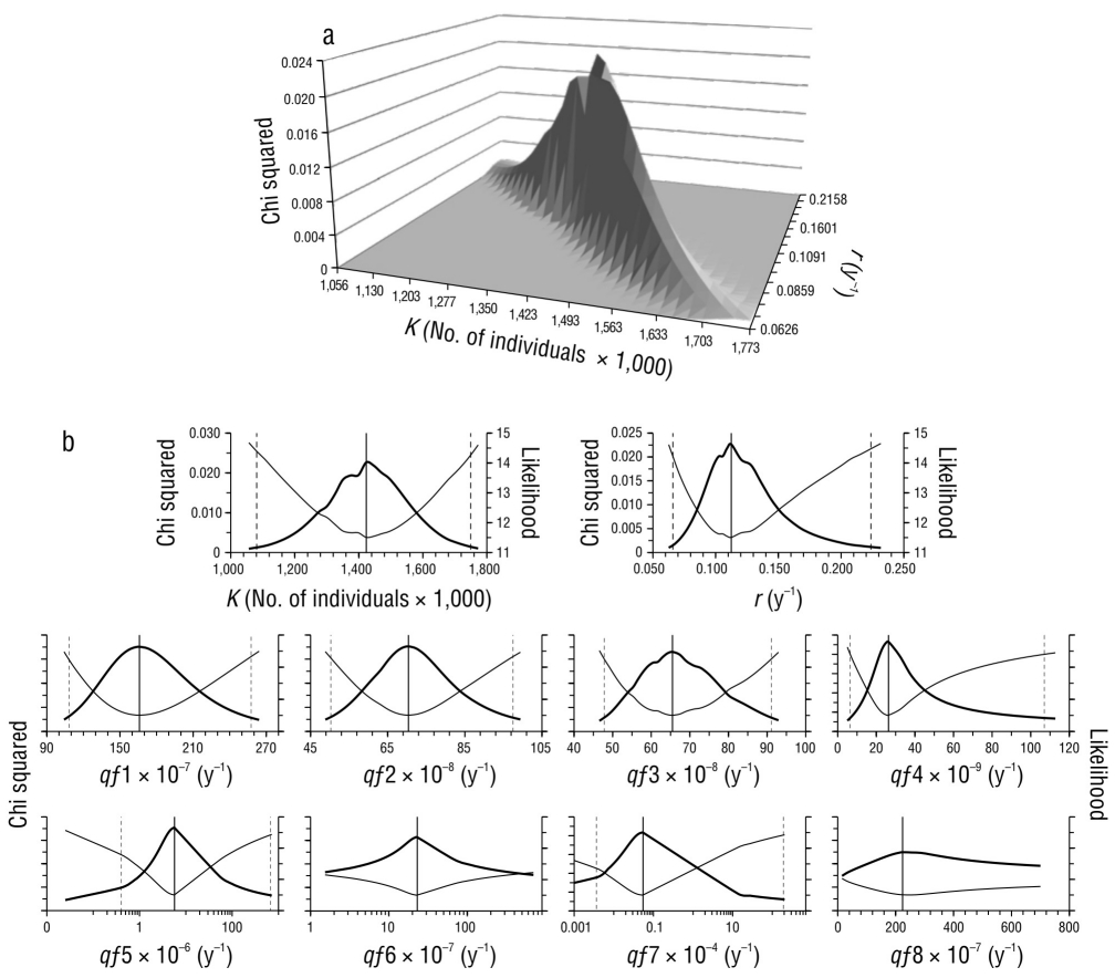
Figure 3 Goodness of the fit to the dynamic abundance model. (a) Likelihood response surface with combinations of carrying capacity (K) and intrinsic growth rate (r). (b) Likelihood profile (thin line) and chi-square (thick line) of K, r, and fleet-specific catchability (qf1-qf8). The vertical lines represent the maximum likelihood (solid line) and the limits of its confidence interval (α = 0.05, broken lines).
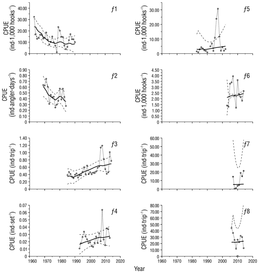
Figure 4 Catch per unit of effort (CPUE) by fleet (f 1-f 8). Observed values (dotted line with circles) and estimated values (thick solid line) with their confidence intervals (α = 0.05: broken lines) are shown. The lower intervals of fleets f 5, f 7, and f 8 only contain negative values and are not shown in the graphs.
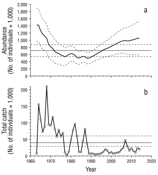
Figure 5 Outputs of the population model for striped marlin. (a) Reconstruction of abundance by year. (b) Total catches recorded per year. The horizontal lines in (a) represent abundance when maximum sustainable yield is reached, and those in (b), the maximum sustainable yield. Confidence limits (α = 0.05) are shown with broken lines.
Simulations
After 2014, recreational fleets (f 3) showed the lowest CPUEs in the historical series and accentuated a negative trend that began with the fluctuation recorded from 2007 (Fig. 6a). Between 2010 and 2014, bycatch represented 81.5% of recreational catches; this proportion was taken to estimate the expected catches between 2015 and 2019 and run the first simulation scenario. Under this scenario, the estimated CPUE would continue its upward trend, which differs notably from the observed CPUE (Fig. 6a). The second scenario showed that the best fit of the CPUE was achieved when we added a catch 27 times the catches of recreational fishing, equivalent to 189 × 103 ind·y-1, on average (Fig. 6b). This scenario implied that abundance would have been reduced to below the N MSY, similar to the abundance reached with commercial fleet exploitation (f 1) between 1963 and 1990 (Fig. 6c).
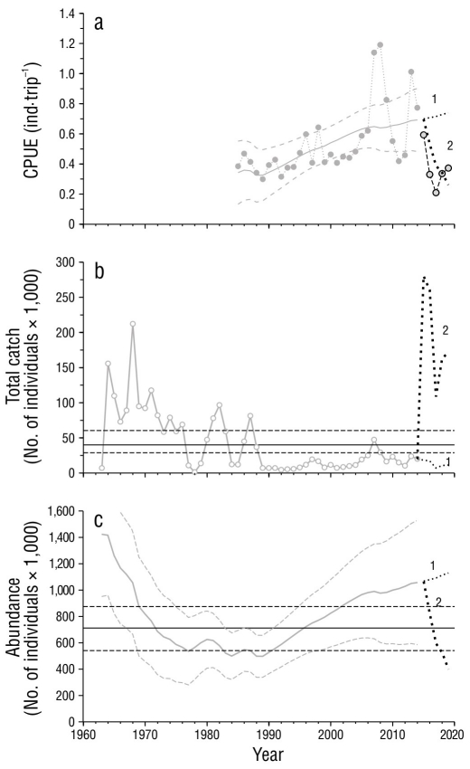
Figure 6 Simulations of scenarios 1 and 2 defined in the Materials and Methods section. (a) Observed catch per unit of effort (CPUE) of the recreational fleets (f 3) with emphasis on the period 2015-2019 (thin broken lines with circles) and fitted curves (medium and thick dotted lines) according to the run scenario. (b) Total catches required to run the simulation scenarios (medium and thick dotted lines). (c) Estimated abundance according to the run scenario. The horizontal lines in (b) represent the maximum sustainable yield, and those in (c), the abundance when the maximum sustainable yield is reached. Confidence limits (α = 0.05) are shown with broken lines.
DISCUSSION
The dynamic model of abundance in this study represented an alternative because the information on the fishery of K. audax is limited and dispersed, given the wide area of distribution of the species and of operation of the fleets. One advantage of the information used in this study is that it came from the region recognized as the population center of this species in the eastern Pacific (Domeier 2006, McDowell and Graves 2008), which maximizes the probability of recording significant changes in the population. One assumption of the model refers to the fact that abundance, in number of individuals, results from the balance between recruitment and immigration versus deaths and emigration. In general, it is assumed that the effect of migration is negligible, either because the proportion of individuals who migrate is low or because immigration is equal to emigration (Hilborn and Walters 1992, Quinn and Deriso 1999, Haddon 2011). In the case of striped marlin, evidence based on mitochondrial DNA shows that there are at least 4 population groups in the Pacific Ocean (Australia, Ecuador, Mexico, and the North Pacific Ocean) between which there is little genetic exchange (McDowell and Graves 2008). This is consistent with satellite tag studies that demonstrate that the striped marlin shows fidelity to regions (Domeier 2006) and spawning sites, which include the waters near the Baja California Peninsula and the mouth of the Gulf of California (González-Armas et al. 2006); this emphasizes the lack of mixing between regions. There is evidence of a population group of striped marlin in the Pacific off Mexico for which migration is not an important factor, and we can assume that its abundance is mainly due to the balance between recruitment and mortality. For mortality, fishing is considered and, with it, the key assumption of constant catchability. Catchability is a parameter linked to the behavior of fishing fleets and is one of the most important sources of variation when assessing a stock (Hilborn and Walters 1992). Klett-Traulsen and Aguilar-Ibarra (2001) highlighted the wide variation in the abundance index (Î t ) of commercial fleets towards the last decade in which they operated (1980-1990), which coincides with the application of regulatory changes that could have affected catchability, such as the establishment of the EEZ of Mexico (Squire 1987) and 2 exclusion zones for commercial billfish fishing at the mouth of the Gulf of California and the Gulf of Tehuantepec (DOF 1987). With these measures, changes occurred in the composition of the fleets and in the fishing areas; therefore, it was not possible to identify whether the variation in the index was due to changes in catchability or effective changes in abundance. The incorporation of the recreational fleets f 2 and f 3 in this study shows that their indices (Î t,f ) had trends and fluctuations similar to those of the commercial fleets f 1 during the period in which they operated simultaneously. Squire (1987) also found a correlation between the CPUEs of commercial fleets and those of recreational fleets between 1969 and 1976 and considered that the index of the recreational fleet could represent the abundance of striped marlin, even in a larger area than its area of influence. Given the consistency in the fluctuations and trends of these fleets, we can assert that the independent indices of each fleet (Î t,f ) seem to respond to a common signal. Considering that recreational fleets operate in more restricted areas than commercial fleets, regulatory measures that could affect the catchability of commercial fleets could hardly affect recreational fleets in the same way. Therefore, the common response signal is more likely to be associated with effective changes in abundance than with catchability.
Although the model explains only a proportion of the variability in the indices of abundance, this proportion is statistically significant, at least for commercial and recreational fleets. This implies that the resolution of the model is too low to explain short-term changes, but we assume the model is able to record trend changes in population abundance. In this sense, it can be stated that, between 1963 and 2014, the abundance of striped marlin went through 3 stages with different trends: a decreasing trend from 1964 to 1977, associated with the effort of commercial fleets (f 1) that exceeded the E MSY and produced catches above the MSY during that entire period; a stable trend from 1977 to 1990 with low abundance, lower than the N MSY, associated with the reduction of the effort by commercial fleets and catches in general, although there were still years in which the catches recorded were higher than the MSY; and an increasing trend after 1990, motivated mainly by the cessation of operations of commercial fleets (f 1). However, according to the fitted model, the increase in population abundance has been progressively slower and, in part, is correlated with the growth of recreational fishing between 1995 and 2007, when the number of trips and catches were increasingly higher. Furthermore, in the same period, bycatch tended to increase, which seems to have also contributed to the population growth slowing down in the last years recorded (2008-2014). These results are broadly consistent with other striped marlin assessments that have a wider geographic coverage (Fig. 1a), which spans the eastern Pacific Ocean (Hinton and Bayliff 2002, Hinton and Maunder 2004, Hinton 2009). Hinton and Maunder (2009) presented the most recent assessment, in which they integrated information from a large area that extends east of the 145° W meridian, between the parallels 5° S and 45° N; these authors used the Stock Synthesis statistical model (Methot 2009), and their results confirmed what was reported in previous assessments: the abundance of striped marlin in the eastern Pacific Ocean is at or above the level expected to obtain the MSY, under a lower fishing effort than would be expected to obtain the MSY and with no indication that the effort could be increased; therefore, it is considered that striped marlin in the eastern Pacific Ocean maintain a biologically acceptable population condition (Hinton and Bayliff 2002, Hinton and Maunder 2004, Hinton 2009).
According to our study, the state of production and abundance seems to be true only until 2014. After this year and until 2019, the CPUE of recreational fleets (f 3) showed a decreasing trend, and inferences made from these fleets indicated that the mortality required to explain this trend change is equivalent to 26 times the catches recorded in the same period, that is, an average mortality of 196,000 ind·y-1. This amount is only comparable with those of the period of greatest exploitation of striped marlin (1963-1990), when the largest catches in the historical series were recorded. In that period, the highest average catches for 5 consecutive years occurred between 1964 and 1968, when average catches of 128,000 ind·y-1 were recorded. It is possible to consider that a mortality as high as that estimated for the most recent years is evidence that there is an incomplete record of catches. This is a frequent issue in the analysis of fisheries, among other things, because of logistical problems, inaccessibility to landing sites, or poor fishing management practices (Cisneros-Montemayor et al. 2013), and the case of the striped marlin fishery is no exception (Hinton and Maunder 2009). Incomplete records are an important source of uncertainty in any fishery assessment; in the case of Mexico landings are estimated to be up to double the official records (Cisneros-Montemayor et al. 2013). In this context, the mortality estimated through the simulations is notably greater than double the recorded landings of striped marlin; therefore, mortality seems too large to attribute it exclusively to non-updated bycatch or even to unreported, illegal, or unregulated catches.
For different species of top predators in the Pacific Ocean, studies have found that the variability of biomass in stocks cannot be completely attributed to fishing (Sibert et al. 2006). There is a particular case with another pelagic species, the jumbo squid (Dosidicus gigas) in the Gulf of California. After a period of high abundance (1996-2010) in which around 75,000 t·y-1 were caught, on average, with peaks exceeding 100,000 t, a decline occurred between 2011 and 2014, with average catches of 34,000 t·y-1, and records since 2015 show average catches of 1,500 t·y-1 (SEMARNAP 1999; CONAPESCA 2010, 2018). Although the effect of fishing cannot be ruled out, there is evidence that this decline in squid is also associated with an increasingly hot pelagic habitat, with less chlorophyll a and considerably low upwelling in the central region of the Gulf of California near the port of Guaymas (Robinson et al. 2013). The case of the jumbo squid is relevant for the analysis in this work for at least 2 reasons. First, like the jumbo squid, the striped marlin is among the species with the highest body growth rate (Markaida et al. 2004, Kopf et al. 2011); therefore, the population dynamics of these species depend, to a large extent, on the trophic conditions of the environment they inhabit and also share (Abitia-Cárdnas et al. 2002, Bazzino et al. 2010, Robinson et al. 2013). Second, the jumbo squid is an important component in the diet of striped marlin (Abitia-Cárdenas et al. 1997, 2002, 2011). Although the analysis by Robinson et al. (2013) focuses on the central region of the Gulf of California, the evidence suggests that the conditions that affected upwelling were not restricted only to the Guaymas region and could have been a process of greater geographic scope, which encompassed the entire Gulf of California. According to the historical series of the coastal upwelling index (CUI) (Bakun 1973, 1975), estimated for the point located at the mouth of the Gulf of California (21° N, 107° W) (Fig. 7)1, a very similar pattern of variation to that recorded by Robinson et al. (2013) for the central Gulf of California region was observed. Before 2003, positive values of CUI predominated, despite showing values with wide oscillations. Conversely, between October 2003 and July 2004, the CUI showed negative values, with an average close to -300 m3·s-1 per 100 m of coastline, and subsequently, values remained negative, with an average close to -30 m3·s-1 per 100 m of coastline until 2010. Undoubtedly, more in-depth analyses are required to understand the mechanisms through which upwelling can affect a particular species in the food web; however, the variation of the CUI described above coincides with the period in which the striped marlin index of abundance showed large fluctuations (2007-2011) and seems to mark the change in the trend of the same index (Fig. 6). The temporal correspondence of these results offers us the basis to hypothesize that the striped marlin population could be under unfavorable trophic conditions that have favored greater natural mortality, which could be a factor, in addition to catches, that helps explain the recent negative trend in striped marlin abundance.

Figure 7 Coastal upwelling index for the position located at the mouth of the Gulf of California (21° N, 107° W). Data estimated by the Environmental Research Division (NOAA-SWFSC) and available at: https://oceanview.pfeg.noaa.gov/products/upwelling/bakun.
In terms of management, this implies that, although the different fleets analyzed operate below the MSY and E MSY levels, the abundance of striped marlin could be below the N MSY. According to the analyses, this state seems to be strongly influenced by the limiting trophic conditions to which striped marlin are subjected; consequently, it is difficult to think of a management measure that could have a direct impact. However, management decisions can be made to mitigate environmental pressure on this species. Any management measure that helps to significantly reduce fishing mortality would help this purpose. Among other alternatives, the strengthening of the catch-release practice in recreational fishing and the reduction of the bycatch quotas that are currently in force in Mexican legislation are management measures that could be applied simultaneously to the 2 main sources of mortality that can be influenced through the management of the fishery of striped marlin.

