


 texto en
  Inglés (pdf)
 Artículo en XML
 Referencias del artículo
 Enviar artículo por email
 Citado por SciELO
  Similares en
SciELO
Similares en
SciELO 
 Permalink
Introduction
Eddies are very common structures in the ocean that have a significant impact on the transport of mass and properties such as heat and salt. For instance, eddies that detach from the Loop Current (LC) transport Caribbean water across the Gulf of Mexico (GM) (Nowlin et al. 1998, Oey et al. 2005, Tenreiro et al. 2018). In addition to increasing productivity through upwelling mechanisms (Hamilton and Lee 2005), eddies have been shown to modulate chlorophyll distribution through horizontal advection (Chelton et al. 2011a). Eddies can also affect the distribution and transport of plankton and fish larvae (Lobel and Robinson 1988, Sánchez-Velasco et al. 2013, Condie and Condie 2016).
The general circulation in the GM is anticyclonic and its dynamics is influenced by the LC (Elliott 1982, Vidal et al. 1994, Zavala-Hidalgo et al. 2014, Meunier et al. 2018). The LC is an intense current that enters the GM through the Strait of Yucatán, extends into the north of the GM, and veers east to exit through the Straits of Florida (Andrade-Canto et al. 2013). It gets its name from the loop shape it takes inside the GM. The LC sheds large anticyclonic eddies measuring up to 300 km (Nowlin et al. 1998, Oey et al. 2005) at irregular intervals, ranging from 15 d to 18 months (Andrade-Canto et al. 2013). Usually, eddies that detach from the LC influence circulation, hydrographic properties, and water masses in the GM. These eddies moved west until impacting against the slope of the western shelf of the GM, where they exchange momentum with their surroundings and generate coastal currents (Biggs et al. 1996, Ohlmann and Niiler 2005), as well as generating eddies upon their interaction with the coast (Vidal et al. 1994) and other eddies (Hamilton et al. 1999) in the region.
The northwestern GM (NWGM) (Fig. 1) is a highly dynamic region with a large number of eddies (Merrell and Morrison 1981; Vidal et al. 1992, 1994; Hamilton 2007). Circulation there is dominated by cyclonic and anticyclonic eddies of widely variable sizes, periods, and durations. Usually, several eddies occur simultaneously (Hamilton 2007). Furthermore, this region contains eddies that are generated independently of the eddies that are shed from the LC (Hamilton 2007).
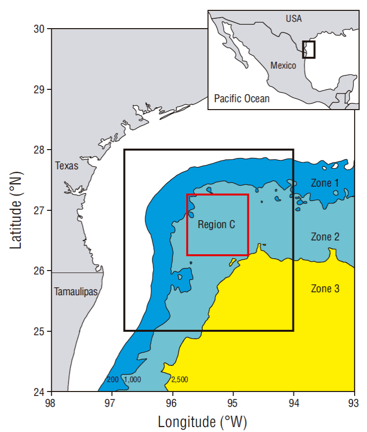
Figure 1 Map of the Gulf of Mexico showing the location of the study area (black square). The black curves represent bathymetry and the red square delimits region C. The zones are represented by the solid colors (see main text for details).
NWGM eddies have been studied using hydrography (Hamilton 1992, Hamilton et al. 2002), drifters (Ohlmann et al. 2001), anchored buoys (Hamilton and Lee 2005), satellite altimetry-derived sea level anomalies (Leben 2005), and even combinations of different methods (Hamilton 2007). Different studies have defined the morphological characteristics of these eddies; however, these studies have assumed that the water mass contained within them is always the same (Chelton et al. 2011b). Beron-Vera et al. (2008) showed that eddy boundaries, obtained through Eulerian methods as sea surface height (SSH) contours or Okubo-Weiss parameters (Okubo 1970, Weiss 1991), generally deform within a few days and, therefore, part of the mass enclosed by these boundaries disperses throughout the surrounding medium. In addition, several studies have shown that eddies have limited capacity to transport mass because they exchange water with their surroundings in their paths (e.g., Biggs et al. 1996, Lipphardt et al. 2008, Wang et al. 2016). In particular, Lipphardt et al. (2008) showed that a large portion of the original core of the Millennium eddy (which occurred during the year 2001) dispersed over the western GM and that this core contained water from the western gulf and not just water from the Caribbean. Therefore, in order to analyze the transport capacity of eddies, it is advisable to study them from a Lagrangian point of view so that processes that are difficult to detect with SSH streamlines or contours can be distinguished (Lipphardt et al. 2008; Beron-Vera et al. 2008, 2013).
Few studies have quantified how long are eddies capable of transporting mass and preserving their properties (d’Ovidio et al. 2013, Condie and Condie 2016, Cetina-Heredia et al. 2019). This topic is of particular interest in the NWGM, given that ocean dynamics in the region are influenced by a large number of eddies (Andrade-Canto et al. 2013, Meunier et al. 2018). In addition, the oil industry carries out intensive work in this region and is expected to expand to deeper waters. An oil spill can cost millions of dollars in losses and environmental damage, as in the case of the Deepwater Horizon oil spill (e.g., Smith et al. 2011). In the event of an oil spill in the NWGM, it is important to assess the effect that eddies could have on the retention and dispersion of oil in this region. This information can be used to make predictions in terms of retention times.
This study identifies eddies present in the NWGM between January 1993 and December 2016. It determines eddy boundaries, their morphological characteristics, how long were they able to transport a body of water within them (coherence time), and the percentage of mass they retained during that time. The method proposed by Haller et al. (2016), which defines eddies as rotationally coherent Lagrangian vortices, is used for this purpose.
Materials and methods
Data and coherent eddy detection
Eddy detection is done from the field of surface geostrophic currents
where g is the gravitational acceleration, f = 2Ω sin λ is the Coriolis parameter, Ω is the rotational angular velocity of the Earth,
The eddy detection method used in this study is based on the computation of the Lagrangian-averaged vorticity deviation (LAVD) field. The LAVD field is a dynamically consistent and objective measure of bulk material rotation relative to the spatial mean rotation of the fluid volume (Haller et al. 2016). This method objectively identifies material tubes along which small volumes of fluid experience the same net rotation within a time interval [t 0 , t τ ] relative to the mean rigid-body rotation of the fluid (Haller et al. 2016). Eddy boundaries can therefore be clearly detected. These boundaries do not show filamentation and the interior of the eddy does not show advective mixing with its surroundings (Haller et al. 2016).
From the geostrophic velocity field, the trajectory of the fluid particles can be obtained by solving
which defines the flow map
which tracks the particles from their initial position x
0
at the initial time, t
0
, to a later position
The relative vorticity ω of the particles that belong to the flow map is calculated for each instant of time as follows:
and the LAVD field is mathematically defined as follows:
where
Considering the definition of LAVD, an eddy contains a nested family of LAVD level surfaces, with maximum values at the center (Haller et al. 2016). The outermost ring of this family of nested curves (limit ring) defines the boundary of the set of particles that remain conjoined. They all rotate at the same mean rotation rate as if they were the surface of a rigid body during the integration time for which the LAVD field was calculated.
Particle advection was carried out using an initial mesh with a resolution of 1/32º. The trajectory of the particles is determined using the fourth/fifth order Runge-Kutta method with an adaptive time step and a tricubic interpolation method. The LAVD fields are calculated using the vorticity of the advected particles (equation 5).
The eddy identification process was carried out every 15 d from 01 January 1993 to 01 December 2016. For each identification process, LAVD fields were calculated using forward-in-time integrations from an initial time t 0 to a final integration time t = t 0 + τ, where τ ranges from 15 d to 120 d in daily intervals. Maximum integration time (τ = 120 d) was set by preliminary tests that indicated that NWGM eddies rarely maintain their coherence for over 120 d.
Eddies were identified following the recommendations of Haller et al. (2016) and Abernathey and Haller (2018). The main steps and criteria used are listed below:
The maxima of each LAVD field were detected.
From each LAVD field, the outermost closed contour that satisfied the 0.01 convexity tolerance was extracted.
Limit rings with radii smaller than 22 km were discarded.
Each ring was advected from time t 0 to τ. Rings with L τ /L 0 < 1.1 were considered to be coherent at time τ, where L 0 and Lτ are the perimeter of the ring at the beginning and end of advection, respectively.
To ensure that eddies were counted only once during their coherence period, in each identification process the centroids of the newly detected eddies were verified to fall outside the boundary ring of the eddies detected in the previous process.
The boundary of an eddy is the limit ring obtained from the LAVD field computed with τ = 15 d. Henceforth, it is referred to as the boundary ring (Rb). From each LAVD field with 15 < τ ≤ 120 d, the concentric boundary rings with radii decreasing toward the center were determined. The last ring that can be detected delimits the core of the eddy and is denominated coherence ring (Rc) (Fig. 2).
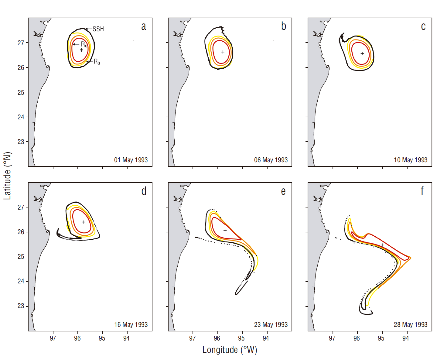
Figure 2 Example of cyclonic eddy detection. The sequence from (a) to (f) represents the advected sea surface height contour and limit rings computed from the Lagrangian-averaged vorticity deviation fields. The cross represents the centroid of the coherence ring (Rc). Rb, boundary ring; SSH, sea surface height.
Eddy characteristics
Bathymetry can affect eddy behavior and characteristics (Lipphardt et al. 2008). For the analysis, the study area was therefore divided into 3 zones, a shallow zone (zone 1) with depths down to 1,000 m, an intermediate zone (zone 2) with depths between 1,000 and 2,500 m, and a deep zone (zone 3) with depths over 2,500 m (Fig. 1).
The initial position of the eddy is defined as the centroid of Rb. The distances from the centroid to each point along the boundary define a set of radii that define its characteristics. The trajectory of the eddy is obtained from the position of the centroid of Rc at each instance of time. Because only mesoscale eddies were considered in this study, Rc had to be larger than ~22 km, the baroclinic Rossby radius of deformation for NWGM (Hamilton 2007).
The angular velocity, σ, is calculated as follows:
where Θ is the angular displacement, V the mean tangential velocity of particles on the eddy boundary, and
The coherence time for each eddy corresponds to the time τ at which Rc was obtained. As an example, Figure 2 shows the temporal evolution of the SSH contour, the Rb (τ = 15), a limit ring for τ = 18, and the Rc (τ = 22) of a NWGM eddy from its detection to 5 d after losing its coherence (see supplementary material: the animation on the online version [Animation S1] or the sequence of figures in this document [Fig. S1]). This example shows that the SSH contour rapidly becomes filamented and that some of its particles disperse to the west, while the coherent part of the eddy detected with the LAVD method, delimited by Rc, remains coherent for 22 d. When Rc filamentation occurs (Fig. 2f), loss of eddy coherence becomes evident.
The percentage of the mass that is preserved at coherence time, L, is estimated as follows:
where
Results
Eddy identification in the northwestern Gulf of Mexico
In the analysis of the 23 years, a total of 254 eddies were identified in the NWGM, 181 of which were cyclonic and 73 anticyclonic (Table 1). There was a notorious predominance of cyclonic over anticyclonic eddies, with a ratio of 2.5:1.0. Cyclonic eddies were present 80.5% of the time in the study period, whereas anticyclonic eddies were present only 27.7% of the time (Table 1); that is, cyclonic eddies were present almost 3 times longer than anticyclonic eddies. The ratio of cyclonic to anticyclonic eddies was 3.3:1.0 in zone 1, 2.5:1.0 in zone 2, and 1.8:1.0 in zone 3. The density of eddies per 10,000 km2 in zones 1, 2, and 3 was 9, 29, and 18 for cyclonic eddies and 3, 11, and 10 for anticyclonic eddies, respectively.
Table 1 Number and characteristics of eddies detected with a Lagrangian method in the northwestern Gulf of Mexico (NWGM) from 1993 to 2016.
| Type | Description | Zone 1 | Zone 2 | Zone 3 | NWGM |
| Cyclones | Quantity | 35 | 112 | 34 | 181 |
| Median radius (km) | 40.48 | 53.18 | 55.53 | 51.52 | |
| Quartile range (km) | 24.17 | 24.93 | 48.72 | 48.72 | |
| Persistence time | - | - | - | 27.77% | |
| Anticyclones | Quantity | 10 | 44 | 19 | 73 |
| Median radius (km) | 43.6 | 50.00 | 68.28 | 52.80 | |
| Quartile range (km) | 20.96 | 26.89 | 27.45 | 28.39 | |
| Persistence time | - | - | - | 80.49% | |
| All | Quantity | 45 | 156 | 53 | 264 |
Approximately 31% of cyclonic eddies in zone 2 were detected in an area of 1º × 1º, marked as Region C in Figure 1. The occurrence of cyclonic eddies in this area is more than twice the occurrence that would be expected if eddies occurred homogeneously throughout the area. Anticyclonic eddies showed a more uniform spatial distribution than their cyclonic counterpart. However, 3 sectors were observed around region C where a greater number of anticyclones occurred: one to the east, another one to the west, and the last one to the southwest (Fig. 3).

Figure 3 Centroids of anticyclones (a) and cyclones (b) for zones 1 (circles), 2 (squares), and 3 (triangles). In (a) and (b) the color bar indicates eddy radius. Also shown are the number of anticyclones (c) and cyclones (d) detected within 0.5 × 0.5º bins. In (c) and (d) the color bar represents the number of detected eddies per bin.
Descriptive statistics of eddies
By detecting eddy boundaries with LAVD, we can define the radius as the distance from the centroid to the boundary of the set of particles that rotate conjointly within the eddy. In zone 1, 75% of the eddies had a radius smaller than 54 km. The median radius was ~40 km, although cyclonic eddies with radii up to ~90 km were detected. In zone 2, 75% of eddies had radii that were less than 65 km and the median radius was ~50 km. By contrast, anticyclonic (cyclonic) eddies in zone 3 were, on average, ~25 km (~15 km) larger than the anticyclones (cyclones) in zone 1 (P value < 0.1 for anticyclones and cyclones). Despite the differences between the median radii for cyclones and anticyclones in zone 3, no significant differences were detected between cyclones and anticyclones when all eddies in the zone were considered, given the variability in eddy radii. Figure 4 (a, b) shows that the radius for eddies in the shallow zone was smaller than that for eddies in the deep zone and it seems to indicate a linear trend. A linear correlation analysis between the radius and the bathymetry associated with eddy centroids showed that bathymetry could moderately influence eddy size (ρ = 0.35, P value < 0.1).
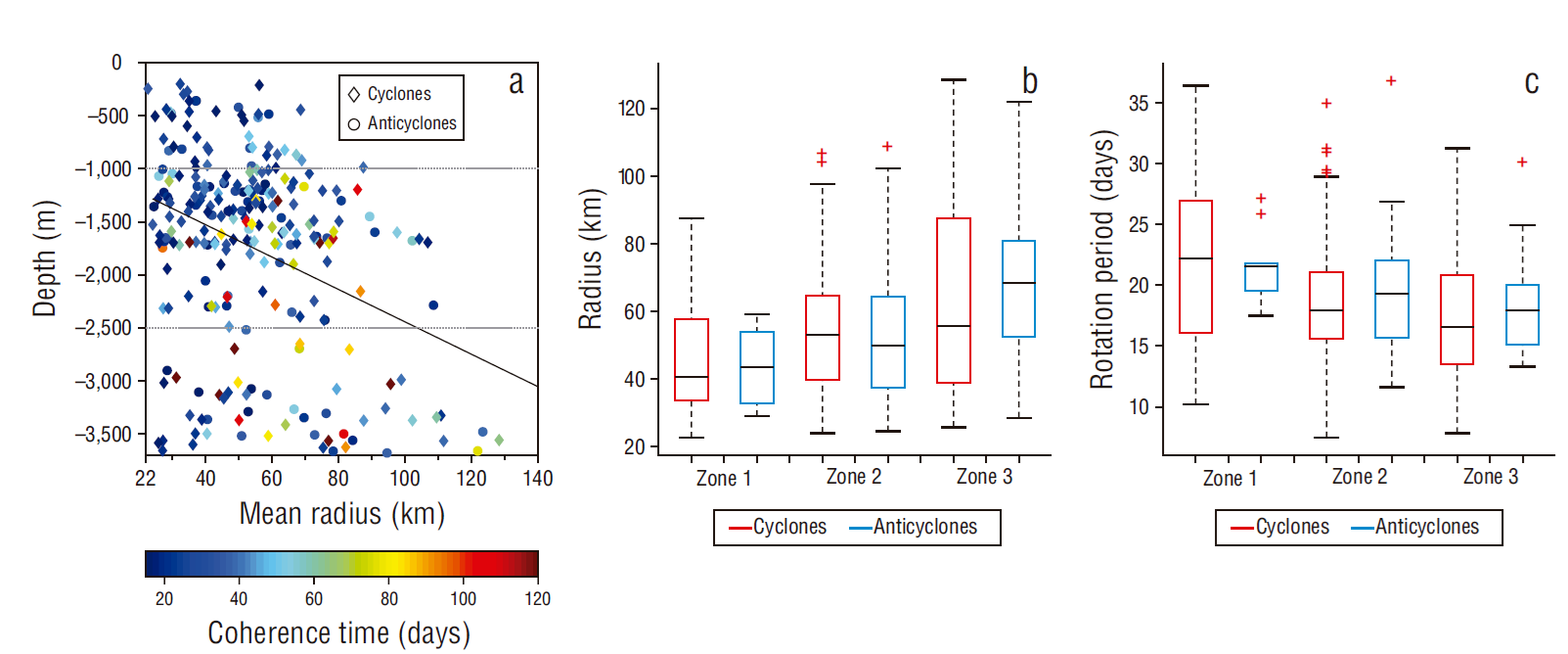
Figure 4 (a) Depth corresponding to the centroid of cyclones (diamonds) and anticyclones (circles) as function of radius. Gray dotted lines delimit the depths for each zone. The linear regression curve is presented in black. (b) Boxplot of radii of eddies in each detection zone. (c) Boxplot of the rotation period of eddies in each detection zone. The upper part of each box represents the 75th percentile and the bottom part the 25th percentile; the black line inside the box is the median, the red crosses identify outliers, and the lower and upper error bars are the minimum and maximum values, respectively.
Eddy rotation periods were also different between the shallow zone and the deep zone (P value < 0.1), but with low linear relationship between them (ρ = 0.25, P value < 0.1) (Fig. 4c). Eddy rotation periods were greater in the shallow zone than in the deep zone. On average, the rotation periods for cyclonic and anticyclonic eddies in zone 3 were, respectively, 7 and 4 d shorter than those corresponding to eddies in zone 1.
Coherence time is the time over which the eddy preserves its core particles within it. When an eddy loses coherence, it stops behaving like a rigid body and it deforms. Consequently, it releases or exchanges particles with the surrounding environment. Most of the eddies detected here have coherence times shorter than 60 d (Fig. 5a). The median coherence time for cyclones increased as the depth corresponding to the position of their centroids increased, from 25 d in zone 1 to approximately 44 d in zone 3 (Fig. 5a). However, the linear correlation between both variables for cyclonic eddies was low (ρ = 0.29, P value < 0.1). Conversely, the coherence time for anticyclones was similar in the 3 depth bands, with a median of around 30 d (Fig. 5a).

Figure 5 (a) Boxplot of coherence times of eddies in each zone. (b) Boxplot of the percentage of preserved mass for eddies in each zone. The upper part of each box represents the 75th and the bottom part the 25th percentile; the black line inside the box is the median, the red crosses identify outliers, and the lower and upper error bars are the minimum and maximum values, respectively.
Eddy contours detected with Lagrangian methods, such as the one used in this study, represent material curves. If we assume that the fluid is incompressible, the area delimited by the eddy contour is proportional to the mass it contains. Therefore, by comparing the initial area of the eddy with the area of Rc (i.e., the L ratio), we can have an idea of the amount of mass that the eddy is able to retain during its coherence period. On average, the eddies detected in the NWGM retained ~60% of their mass throughout their coherence period. In general, there were no differences between cyclonic and anticyclonic eddies except in zone 1, where cyclones had a slight tendency to preserve more mass than eddies in other zones (P value < 0.1). On the other hand, small eddies tended to dissipate as they lost coherence, whereas large eddies were able to regroup and form a new eddy that contained part of the mass of the previous eddy and surrounding water.
Discussion
Eddies in the northwest Gulf of Mexico
Eulerian methods assume that mesoscale eddies, defined from SSH contours or streamlines (Fig. 2), trap and transport water masses for long periods of time, particularly when the rotational speed U (maximum average geostrophic speed of the closed SSH contours within the eddy; Chelton et al. 2011b) is greater than the translation speed c, U/c > 1 (Chelton et al. 2011b). However, the water mass or particles contained within an eddy can pass through the SSH contours (see Fig. 2 and the example at the end of the Descriptive Statistics of eddies section) or streamlines (Lipphardt et al. 2008), and the ability of eddies to transport particles could therefore be incorrectly evaluated (Beron-Vera et al. 2008). Typically, Eulerian detected eddy contours stretch and fold over the course of a couple of weeks, even if U/c > 1, which results in eddy filamentation (i.e., loss of coherence; Beron-Vera et al. 2013).
Eddy detection with Eulerian methods is limited by the resolution of input data. In this regard, Chelton et al. (2011b) and Le Vu et al. (2018) recommend excluding eddies with radii smaller than 50 km when detection is done using AVISO data with resolution of 1/4º. By contrast, Abernathey and Haller (2018), after applying the LAVD methodology, excluded eddies with radii smaller than 15 km from 1/6º resolution data, and Haller et al. (2016) excluded eddies with radii smaller than 20 km from 1/4º AVISO data. Detecting eddies with radii smaller than 50 km is possible because the LAVD method does not depend on an instantaneous description of velocity or SSH fields. This method is based on the integral of the vorticity of advected particles over time (Haller et al. 2016).
On the other hand, coherent Lagrangian eddies, like the ones detected with the LAVD method, generally have a radius that is smaller than the radius of their Eulerian counterpart (Beron-Vera et al 2008, 2015; Wang et al. 2016; Abernathey and Haller 2018) (Fig. 2). Therefore, to get an idea of the reliability of detecting small eddies with the LAVD method, they were compared with their Eulerian counterpart, which was detected from closed SSH contours. All Lagrangian eddies with radii smaller than 50 km had a Eulerian radii larger than 40 km, and 95% had Eulerian radii larger than 50 km.
According to our analysis, in this region there are more cyclonic than anticyclonic eddies (2.5:1.0). This is consistent with what can be inferred from Figures 3a and 4a in Hamilton (2007). Region C was delimited in zone 2; almost 30% more cyclonic eddies occurred in this region compared to the rest of the zone (Figs. 1, 3d). This allows us to assume that if an oil spill were to occur in this region, it is ~30% more likely that the oil will be trapped and transported inside an eddy as long as the eddy maintains its coherence. In addition, coherent cyclonic eddies have the ability to attract particles whose densities are lower than the density of water (Beron-Vera et al. 2015). Specifically, the LAVD centers are the attractants in these eddies (Haller et al. 2016) and, therefore, it can be hypothesized that a light hydrocarbon (density equal to or less than that of water) will possibly be attracted to the LAVD center of the cyclonic eddy and that this hydrocarbon will be transported until the eddy loses its coherence.
Eddy characteristics
Defining eddy boundaries properly is a challenging task because it depends on the criteria used for doing so (e.g., SSH contours, streamlines, temperature contours, buoy trajectories, etc.). In this study, the eddy boundary (Rb) and Rc, which coincides with the eddy core boundary, were determined using the LAVD method. Together, these 2 rings make it possible to define characteristics of great interest, such as retention time and percentage of retained mass, which are key variables in the dispersion of light particles such as hydrocarbons.
Previous studies such as those by Hamilton (1992, 2007) indicate that some NWGM eddies can have Eulerian durations of up to 6 months, without considering retention/coherence times. A similar study conducted off the east coast of Australia showed that particle retention times within eddies were 24 and 27 d for anticyclones and cyclones, respectively (Cetina-Heredia et al. 2019). Additionally, studies of eddies forming from the retroflection of the Agulhas Current revealed coherence times between 3 months and 1 year (Wang et al. 2015) and even eddies with coherence times greater than a year and a half (Beron-Vera et al. 2013, Wang et al. 2016). The great variability in coherence times allows us to assume that there is no global pattern and that each zone requires particular analysis.
NWGM eddies retain ~60% of their mass until they lose coherence. Similar studies have shown that eddies detaching from the retroflection of the Agulhas Current only retain 30% of the mass they initially contained (Wang et al. 2015, 2016), suggesting that eddies have a limited capacity to transport mass during their life span. This reinforces the importance of studying eddy mass transport using Lagrangian methods, such as the one used in the present study.
The simultaneous presence of various eddies was observed on several occasions. It is possible that some of these cases correspond to the dipoles/tripoles that have been described in the area (Merrell and Morrison 1981, Merrell and Vázquez 1983, Lipphardt et al. 2008). These structures can favor the interaction among eddies and, consequently, loss of coherence. However, this topic would have to be studied separately with the objective of determining what happens to eddy water mass properties when dipoles or tripoles occur.
These results and their analysis may be of great interest to evaluate transport in the case of oil spills or to study the transport of biota by eddies in the region. For example, knowing coherence times and the percentage of mass retained by NWGM eddies is the beginning for making assertive decisions in the event of an oil spill. Because of this, the relationship between the peripheral radius Rb and its core Rc is a practical way to estimate the percentage of mass retained by an eddy from the moment it is detected to the moment it loses coherence. The eddy parameters reported here can be used as the basis for validating numerical models of circulation in the NWGM.
In summary, the median radii of the NWGM eddies detected in this study vary from ~40 km in the shallowest zone to ~70 km in the deepest zone. NWGM eddies retain approximately 60% of their initial mass from the moment of their detection until the loss of their coherence. Also, the eddies observed in the region rarely retained their initial mass for more than 60 d. In particular, on average, cyclonic eddies in the region retain their initial mass for ~33 d, whereas anticyclonic eddies retain it for ~26 d. Finally, there is a region, centered between 94.75º W and 26.75º N, where approximately 30% of the total number of cyclonic eddies detected between the 1,000- and 2,500-m isobaths occurred.


