


 nueva página del texto (beta)
 Inglés (pdf)
 Artículo en XML
 Referencias del artículo
 Enviar artículo por email
 Citado por SciELO
  Similares en
SciELO
Similares en
SciELO 
 Permalink
Introduction
The California Current System (CCS) is a very large transitional area that forms the eastern boundary of the North Pacific Gyre, with the confluence of Subarctic Water, Tropical Surface Water, and Subtropical Surface Water (Hickey 1998). It basically consists of a wide (>500 km) equatorward surface (up to 300 m depth) current and a poleward subsurface flow at the edge of the continental shelf (Lynn and Simpson 1987). Equatorial Water penetrates the system through the southern limit in the form of a subsurface countercurrent near the coast (200 m depth). Researchers thought this countercurrent occurred as a narrow poleward surface flow during part of autumn and winter (Lynn and Simpson 1987), but the surface and subsurface countercurrents are independent phenomena (Durazo 2015). The CCS is characterized by a large number of meanders, eddies, filaments, fronts, and mesoscale structures that span for tens to hundreds of kilometers offshore and last from days to months (Hickey 1998, Espinosa-Carreón et al. 2004, Barocio-León et al. 2007).
In the CCS, wind-induced upwelling events, which show seasonal variability, bring cold, nutrient-rich waters along the coast, from Washington to Baja California (Huyer 1983). This results in phytoplankton biomass (chlorophyll a concentration, Chl) and phytoplankton production (PP) gradients, with high values in the inshore area and a clear decrease towards the offshore area (Fargion et al. 1993, Arroyo-Loranca et al. 2015). The high Chl and PP values in the inshore area (0-120 km from the coast) sustain high populations abundances of marine mammals and birds, and important fisheries. However, the CCS is influenced by El Niño/Southern Oscillation (ENSO) events that are associated with an increase of sea surface temperature (SST) and a decrease of Chl and PP (Putt and Prézelin 1985; Torres-Moye and Alvarez-Borrego 1987; Reid 1988; Lynn et al. 1998; Kahru and Mitchell 2000, 2002). By contrast, events with anomalously low SSTs (La Niña) may have the opposite effect, with relatively high Chl and PP.
An anomalous warming in the North Pacific (known by the nickname “The Blob”) led to major disturbances in the California Current ecosystem (Gentemann et al. 2017). The Blob, which was a very large mass of relatively warm Pacific water off the western coast of North America, appeared for the first time in the Gulf of Alaska in autumn 2013 (Bond et al. 2015), and its influence on the southernmost part of the CCS lasted until the end of November 2015 (see SST anomaly charts in NOAA 2017a). This marine heat wave persisted throughout 2013-2015 because of the atmospheric teleconnections that spanned the entire North Pacific (Di Lorenzo and Mantua 2016). In the area off the Baja California Peninsula, SST in coastal waters off northern Baja California in October 2014 was ~6 ºC above the maximum temperatures of other years in the period 2008-2014 (Coronado-Álvarez et al. 2017). Similar anomalously high SST values were also recorded for the southernmost latitudes of the peninsula, off Cabo San Lucas (NOAA 2017a).
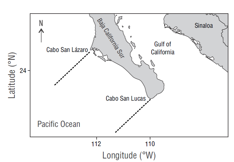
The coastal southernmost part of the CCS has been studied very little. The program Investigaciones Mexicanas de la Corriente de California only covers down to what was line 137 of the California Cooperative Oceanic Fisheries Investigations program, off the southern part of the Gulf of Ulloa (Durazo and Gaxiola-Castro 2010). The main objective of this work is to describe and quantify satellite-derived chlorophyll a (Chlsat) and PP variabilities in 2 contrasting areas, Cabo San Lázaro and Cabo San Lucas (Fig. 1), at seasonal and interannual scales, and to explore the possible forcing agents underlying these variations. The main hypotheses are (1) there are clear inshore-offshore Chlsat and PP gradients, with higher values in the inshore than in the offshore area at both studied sites; (2) inshore Chlsat and PP values are greater off Cabo San Lázaro than off Cabo San Lucas; and (3) the impact of warm interannual events like El Niño is larger off Cabo San Lucas than off Cabo San Lázaro.
Materials and methods
Study areas
The area off Cabo San Lázaro (CSLa) is the southern limit of the Biological Activity Center of the Gulf of Ulloa (Martínez-López and Verdugo-Díaz 2000). The oceanic zone off Magdalena Bay, immediately to the south of CSLa, is dynamically complex; it shows high seasonal and interannual variabilities, and its circulation patterns generate a sequence of eutrophic and oligotrophic conditions (Longhurst et al. 1967, Walsh et al. 1977). Eutrophic conditions occur in March-June and are directly associated with strong winds from the northwest, a well-developed California Current, and maximum upwelling index values (Bakun and Nelson 1977). Oligotrophic conditions occur in September-December and are associated with high-salinity water, which is transported by the surface coastal countercurrent, and with the relaxation of upwelling; July, August, January, and February are considered transition months (Bakun and Nelson 1977).
There is an oceanic front in the area off Cabo San Lucas (CSLu). The front extends from the surface down to 120 m depth, and it is formed by the confluence of different water masses: Gulf of California Water, California Current Water, and Northeast Pacific Subtropical Water (Griffiths 1963). Warsh et al. (1973) identified another water mass that can also contribute to the formation of the front, the northeastern Pacific Subtropical Subsurface Water, located at 50-200 m depth. The Cabo San Lucas Front is present during most of the year, though there are months when it weakens because of the decreasing effect of the California Current. Circulation at the front is affected by the warm gulf water, which moves westward near the coast, and the cold California Current water, which also moves westward but away from shore (Álvarez-Arellano and Molina-Cruz 1984).
PP and Chlsat values have been reported for the area off CSLa: 0.31 g C·m-2·d-1 (from 14C incubations, Longhurst et al. 1967) and up to 4.5 mg·m-3 (data from the Coastal Zone Color Scanner, CZCS; Zuria-Jordán et al. 1995), respectively. These values are the result of upwelling events. When upwelling relaxes by the effect of the surface countercurrent, among other causes, PP and Chlsat values decrease to less than 0.08 g C·m-2·d-1 (from 14C incubations, Gaxiola-Castro and Álvarez-Borrego 1986) and 0.36 mg·m-3 (Zuria-Jordán et al. 1995), respectively. On the other hand, Lara-Lara and Bazán-Guzmán (2005) reported Chl and PP values of 0.32 mg·m-3 and 0.16 g C·m-2·d-1, respectively, for the area off CSLu; here, Chl was measured in water samples and PP by the 14C incubation technique during an oceanographic cruise carried out in January 1999.
Satellite data
Monthly composites of SST and Chlsat from the Moderate Resolution Imaging Spectroradiometer aboard the Aqua satellite (EOS PM) (Aqua-MODIS), for the period from January 2003 to December 2016, were used. These composites (level 3, 9 × 9 km2 pixel size) were obtained from the NASA Ocean Color website (NASA 2017). Data for SST are from day measurements with 11 µm radiation. Imagery for PP (pixel size 18 × 18 km2) was obtained from the Oregon State University Ocean Productivity website (http://www.science.oregonstate.edu/ocean.productivity/index.php). Images were downloaded in .hdr format (Hierarchical Data Format). PP is given as a defined standard product calculated using the Behrenfeld and Falkowsky (1997) vertically generalized productivity model (VGPM). The VGPM is a non-spectral model with homogeneous vertical distribution of biomass and with vertically integrated production. Satellite imagery was processed with the software provided by NASA (SeaDAS v.7.1), which was also obtained from the Ocean Color website (NASA 2017).
Two 300-km long transects, one off CSLa (TCSLa) and the other off CSLu (TCSLu) (Fig. 1), were sampled from the SST, Chlsat, and PP monthly composites to describe the spatial and temporal variations of these properties. In order to describe these temporal variations in detail, time series were generated for each property with their monthly averages for 2 coastal quadrants (18 × 18 km2), one off CSLa and the other off CSLu. A time-series analysis of the 3 variables was performed to characterize the frequencies with the largest contributions to variability.
As a first approximation to the climatology, an “average year” was generated for each property and for each transect. To do this, all data for the Januaries were averaged, and then all data for the Februaries, and so on for each variable and for each transect. Data from at least 30 years are required to generate a real climatology. According to the Chlsat climatology, transects were divided into an inshore area (from the coast to ~110 km) and an offshore area (110-300 km). Also, the year was divided into 2 seasons according to the Chlsat climatology for the inshore area.
Mann-Whitney tests were run to compare Chlsat values between the 2 seasons, separately for inshore (0-110 km) and offshore (110-300 km) waters, for each transect. Mann-Whitney tests were also run to compare inshore and offshore waters, for each transect and for each season; and to compare between transects, separately for inshore and offshore waters and for each season. Hovmöller diagrams were built with SST and Chlsat data from all years.
Results
In general, the “average year” showed clear spatial variations on both transects (Fig. 2). During the first half of the year SST had a monotonic distribution, with low values in the inshore area and high values in the offshore area. However, SST maxima and minima occurred from August through December on TCSLa and in June, July, and December on TCSLu. On TCSLu, SST varied monotonically from August through November but with an inverse gradient, with values decreasing from the inshore to the offshore area. In general, for both transects, the “average year” was divided into 2 seasons: from January to June, with relatively low SSTs (<23 ºC), even in the offshore area; and from July to December, with relatively high SSTs (>23 ºC and up to ~29 ºC), except for December at TCSLa when values were between 22.0 and 23.0 ºC (Fig. 2).
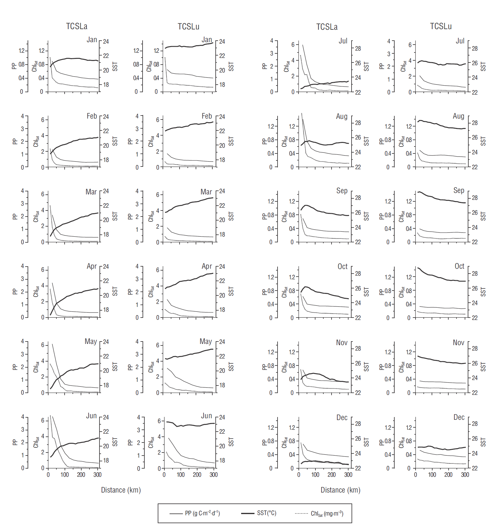
Figure 2 Climatology of 3 variables for the transect off Cabo San Lázaro (TCSLa) and the transect off Cabo San Lucas (TCSLu). The 3 variables are phytoplankton production (PP), satellite-derived chlorophyll a (Chlsat), and sea surface temperature (SST). Note that the scales for Chlsat and PP for January and August-December are different from those for February-July; and the scale for SST for January-June is different from that for July-December.
In the “average year,” SST was clearly greater on TCSLu than on TCSLa. Maximum SST on TCSLa was 27.0 ºC and minimum SST was 17.3 ºC, whereas on TCSLu maximum SST was 28.9 ºC and minimum SST was 20.9 ºC. On both transects SST minima and maxima occurred in the inshore area in April and September, respectively. The SST difference between the inshore and offshore areas was generally >1.0 ºC, with values up to ~3.0 ºC, but during the summer it was as small as ~0.6 ºC. For the offshore area, maxima and minima were, respectively, 25.8 and 20.8 ºC for TCSLa and 27.5 and 22.8 ºC for TCSLu (Fig. 2).
According to the Chlsat spatial distribution for the “average year,” the inshore area can be considered to be from the coast to ~110 km (mainly during May-July) (Fig. 2). In terms of Chlsat and PP climatology, the inshore biological conditions on TCSLa were grouped into 2 seasons: the first from February to August, with the highest value in June (6.6 mg·m-3); and the second from September to January, with lower values than in the first season. The maximum value in the second season was 1.0 mg·m-3 and it occurred in January, in the inshore area. Two seasons were also noted for the TCSLu inshore area: the first from February to July, with the highest value in June (2.0 mg·m-3); and the second from August to January, with lower values (<1.0 mg·m-3, except for a January value from the pixel closest to the coast) than in the first season. The lowest value in the “average year” for both transects was ~0.1 mg·m-3, and it occurred in the offshore area (~250 to 300 km).
The PP plots for the “average year” were very similar to the Chlsat plots (Fig. 2). For both transects, there were 2 defined seasons for PP, as was the case for the Chlsat temporal variation. In the inshore area of both transects, the PP maxima for the first season occurred in June (4.0 and 2.3 g C·m-2·d-1 for TCSLa and TCSLu, respectively), and the PP maxima for the second season occurred in January (0.9 and 0.7 g C·m-2·d-1 for TCSLa and TCSLu, respectively). PP minima for both transects were 0.4 g C·m-2·d-1 for the first season and 0.3 g C·m-2·d-1 for the second season (with the exception of the 0.4 g C·m-2·d-1 values in January), both occurring in the offshore area.
The year-to-year SST variation for both transects had clear seasonal and interannual components. During the studied period, SST on TCSLa ranged from 15.8 ºC (May 2006) to 29.1 ºC (August 2014) in the inshore area and from 19.0 ºC (April 2006) to 28.3 ºC (October 2015) in the offshore area. The SST range for the TCSLu inshore area was 19.3 ºC (April 2004) to 31.0 ºC (September 2015), and that for the TCSLu offshore area was 20.1 ºC (February 2011) to 30.4 ºC (August 2015).
There was an intense SST spatial gradient during the first season of every year, with colder waters in the inshore area than in the offshore area, whereas during the second season waters were relatively warm throughout both transects. Also, waters in the furthest offshore area were warmer during the second season than during the first. Thus, there were clear seasonal SST changes not only in the inshore area but also further offshore on both transects (Fig. 3).
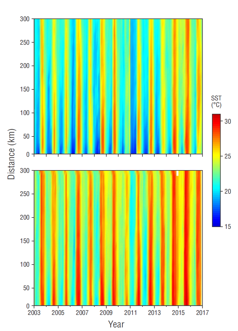
Figure 3 Hovmöller diagrams of sea surface temperature (SST) for the transect off Cabo San Lázaro (upper panel) and the transect off Cabo San Lucas (lower panel). Tick marks on the horizontal axes indicate the beginning of each year.
In the inshore area of both transects SST values in the second season of 2005, 2007, and 2010 tended to be lower than SST values in the second season of other years. They were followed by SST values from the first season of 2006, 2008, and 2011, which were lower than SST values in the first season of other years. This phenomenon was more evident on TCSLa than on TCSLu. These low SST values were recorded along the full extension of the transects, from the coast to the furthest offshore waters, mainly in 2011 (Fig. 3).
On the other hand, for both transects, SST values in the first season of 2010, 2014, 2015, and 2016 tended to be higher than SST values in the first season of other years, yet this phenomenon was more evident on TCSLu than on TCSLa. In 2010 the high SST values in the first season were followed by some of the lowest second-season SST values, and this relative cooling continued into the first season of 2011 throughout both transects. The high SST values in the first season of 2014 and 2015, however, were followed by some of the highest second-season SST values. In 2016 the second-season SSTs went back to “normal” on both transects (Fig. 3).
The largest negative SST anomalies (not illustrated), with respect to our climatology, were down to -4.7 ºC (September 2010) for the TCSLa inshore waters, with relatively large negative anomalies (smaller than -2.4 ºC) throughout the transect. The largest positive SST anomalies for TCSLa were up to +4.0 ºC (May 2015), with relatively large positive anomalies (in most cases greater than +3.0 ºC) throughout the transect. For TCSLu the largest negative SST anomalies were -3.9 ºC (July 2010), with relatively large negative anomalies (smaller than -2.6 ºC in most cases) extending throughout the transect. The largest positive SST anomalies for TCSLu were up to +3.1 ºC (July 2014 and July 2015) in the inshore waters, with anomalies decreasing offshore to less than +2.0 ºC (not illustrated).
In the year-to-year variation, Chlsat and PP values were relatively high in the coastal zone of both transects (≥1.0 mg·m-3 and ≥1.0 g C·m-2·d-1, respectively) in late spring and early summer; these values extended from the coast to 110 km, although very often to only 30-50 km. In the coastal zone, Chlsat and PP variations showed clear seasonal and interannual components (Figs. 4, 5). Sometimes the Chlsat maximum was not adjacent to the coast but between 10 and 40 km from shore. In comparison with the other studied years, the spatial extent of relatively high Chlsat values was larger in 2008, 2011, and 2012 (from the coast to >100 km offshore) on TCSLa, and in 2011, 2012, and 2013 on TCSLu (Fig. 4).
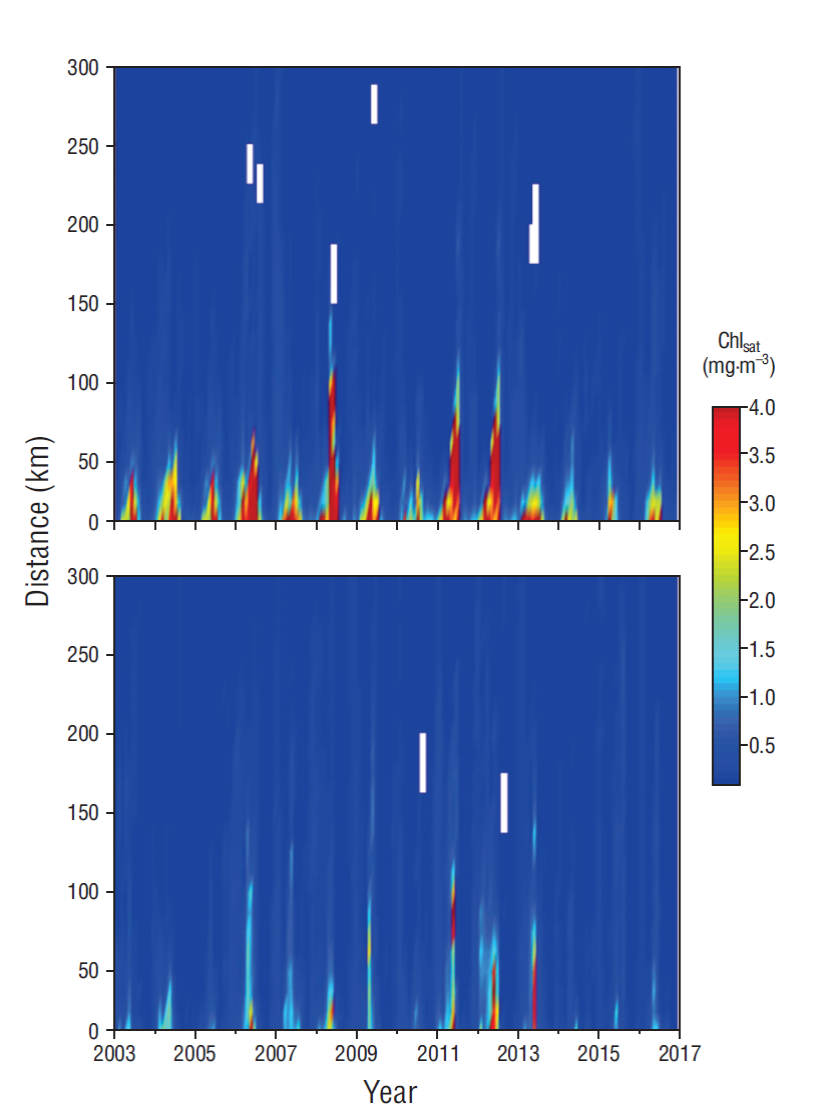
Figure 4 Hovmöller diagrams of satellite-derived chlorophyll a (Chlsat) for the transect off Cabo San Lázaro (upper panel) and the transect off Cabo San Lucas (lower panel). Tick marks on the horizontal axes indicate the beginning of each year.
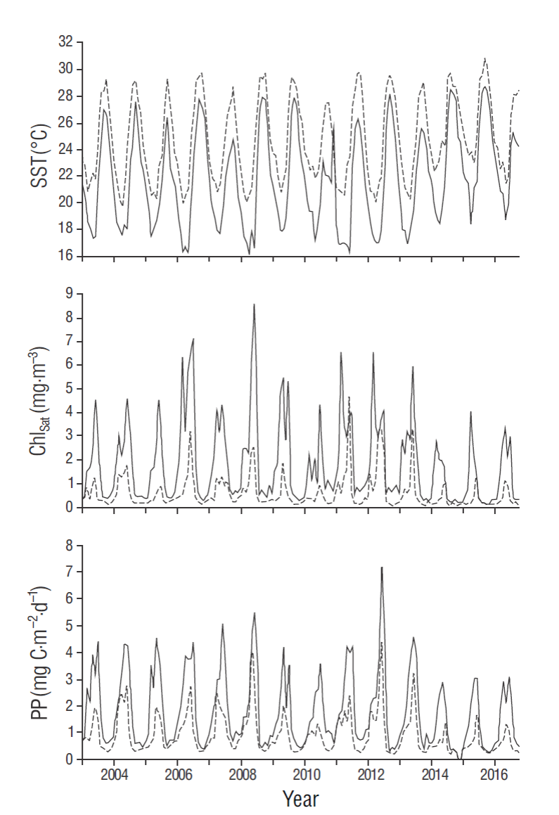
Figure 5 Time series of sea surface temperature (SST), satellite- derived chlorophyll a (Chlsat), and phytoplankton production (PP) in the 18 × 18 km2 coastal quadrants off Cabo San Lázaro (continuous lines) and off Cabo San Lucas (dashed lines). Marks on the horizontal axes indicate the beginning of each year.
In the offshore waters of both transects, yearly Chlsat minima fluctuated between 0.01 and 0.10 mg·m-3 and PP minima between 0.02 and 0.30 g C·m-2·d-1. Also in these waters, Chlsat maxima fluctuated between 0.10 and 0.60 mg·m-3, and PP maxima ranged between 0.40 and 0.70 g C·m-2·d-1. There was no trend for the occurrence of these extreme values at particular times of the year.
Hovmöller diagrams showed greater spatial and temporal variations for Chlsat than for SST in the inshore but not the offshore waters of both transects. The seasonal and interannual Chlsat variations were very clear for the inshore area but not for the offshore area (Fig. 4). The Chlsat inshore values from the first season were much higher, and showed longer duration, on TCSLa than on TCSLu.
With respect to other years in the study period, in the TCSLa inshore waters Chlsat values from the first season were clearly lower (though some >4 mg·m-3) in 2010, 2014, 2015, and 2016, and in the TCSLu inshore waters these values were lower (all <2 mg·m-3) in 2003, 2005, 2010, 2014, 2015, and 2016 (Fig. 4). In the TCSLa inshore waters, Chlsat values from the first season were higher and showed larger spatial and temporal extension in 2006, 2008, 2011, and 2012 than in other years; in 2008 Chlsat values >4 mg·m-3 were detected more than 100 km offshore (Fig. 4). In the TCSLu inshore waters, Chlsat values from the first season were higher, albeit few >4 mg·m-3, and covered a larger spatial extension in 2011, 2012, and 2013 than in other years. On TCSLu relatively high Chlsat values (~2 mg·m-3) were detected even at ~200 km from the coast for several years (2006, 2007, 2009, 2011, 2012, and 2013); in 2011, Chlsat values >4 mg·m-3 were detected at 75-100 km from the coast (Fig. 4).
Results from the Mann-Whitney tests indicate that Chlsat differences were significant in all comparisons, except for the comparison of the offshore Chlsat values from the second season between transects (Table 1). These results indicate that Chlsat values were significantly higher during the first season than during the second season in both zones and on both transects; that the Chlsat values were significantly higher in inshore waters than in offshore waters during both seasons and on both transects; and that the inshore Chlsat values were significantly higher on TCSLa than on TCSLu during both seasons, though the offshore Chlsat values were higher on TCSLa than on TCSLu during the first season but not during the second season.
Table 1 Results of the Mann-Whitney tests comparing paired satellite-derived-chlorophyll-a data sets: TCSLa, transect off Cabo San Lázaro; TCSLu, transect off Cabo San Lucas; CZ, coastal zone; OZ, offshore zone. Bold font indicates significantly different values.
| TCSLa | CZ: First vs second season | n = 1,296 | P < 0.001 |
| OZ: First vs second season | n = 2,154 | P < 0.001 | |
| TCSLu | CZ: First vs second season | n = 1,296 | P < 0.001 |
| OZ: First vs second season | n = 2,156 | P < 0.001 | |
| TCSLa | First season: CZ vs OZ | n = 1,723 | P < 0.001 |
| Second season: CZ vs OZ | n = 1,727 | P < 0.001 | |
| TCSLu | First season: CZ vs OZ | n = 1,728 | P < 0.001 |
| Second season: CZ vs OZ | n = 1,724 | P < 0.001 | |
| CZ | First season: TCSLa vs TCSLu | n = 1,296 | P < 0.001 |
| Second season: TCSLa vs TCSLu | n = 1,296 | P < 0.001 | |
| OZ | First season: TCSLa vs TCSLu | n = 2,155 | P < 0.001 |
| Second season: TCSLa vs TCSLu | n = 2,155 | P = 0.61 |
The SST time series showed that the annual cycle dominated the SST variation in the coastal quadrants off both capes (Fig. 5). Spectral analyses of the time series also showed this (not illustrated). Sea surface temperature was almost always higher off CSLu than off CSLa. In both time series SST maxima occurred at the end of summer and SST minima in spring. For both capes maximum SST values in our study period occurred in September 2015, with 29.8 ºC off CSLa and 31.0 ºC off CSLu. The largest SST seasonal difference for the quadrant off CSLa was ~11.8 ºC and occurred in 2008; the one for the quadrant off CSLu was 9.7 ºC and occurred in 2012. The largest difference between maxima of consecutive years was -3.5 ºC for CSLa and -2.4 ºC for CSLu, both occurring between 2015 and 2016 (Fig. 5).
The Chlsat and PP time series also showed that the annual cycle dominated variations in both coastal quadrants (Fig. 5). The Chlsat and PP time series showed more than one maximum value for several years. In the case of Chlsat, there were 10 years with 2 maxima and 4 years with one for the quadrant off CSLa and 6 years with 2 maxima and 8 years with one for the quadrant off CSLu. PP did not show the same number of years with 2 maxima as Chlsat did; there were 4 years with 2 PP maxima for CSLa and 5 years with 2 PP maxima for CSLu (3 maxima for CSLa in 2003 and 3 maxima for CSLu in 2011). There was a very clear contrast in Chlsat and PP concentrations between the 2 quadrants, with higher values off CSLa than off CSLu (Fig. 5). The first-season Chlsat values were highest in 2008 for CSLa and in 2011 for CSLu (8.6 and 4.7 mg·m-3, respectively). The highest PP values occurred in 2008 for both sites, and they were 5.5 and 4.8 g C·m-2·d-1 for CSLa and CSLu, respectively.
Discussion
The SST, Chlsat, and PP annual cycles on the TCSLa and TCSLu transects (Figs. 2-5) are associated with the dynamics of the CCS. Zuria-Jordán et al. (1995) reported Chlsat values, derived from the CZCS for the area off CSLa, and found them to be higher from February to July than during the rest of the year, similar to what is reported in this study. The California Current and coastal upwelling events intensify in spring and at the beginning of summer, with a strong annual biological signal (Espinosa-Carreón et al. 2004).
According to Lynn and Simpson (1987) and Durazo et al. (2010), in winter the California Current and upwelling events are weak and a surface countercurrent flows near the coast. This winter surface countercurrent should produce higher SST values and lower Chlsat and PP values in late autumn and early winter than in spring and summer. As indicated by Arroyo-Loranca et al. (2015), the surface countercurrent accumulates water near the coast because of the Coriolis effect, thus inhibiting coastal upwelling. On the other hand, coastal upwelling generates a southward surface flux (Mann and Lazier 2006), which inhibits the surface countercurrent to some extent. During the period of weak coastal upwelling (the second season) Chlsat values are often <0.2 mg·m-3 (Figs. 2, 4), indicating oligotrophic conditions in winter and strong seasonal variations.
Santamaría-del-Ángel et al. (1999) used CZCS data from the Gulf of California and concluded that during the nonupwelling season, Chlsat collapses to <0.1 mg·m-3, as was also sometimes the case for the coastal zone off CSLu. On the other hand, Arroyo-Loranca et al. (2015) and Mirabal-Gómez et al. (2017) reported that, respectively, for transects off Punta Eugenia and transects off northern Baja California and La Jolla, California, the lowest Chlsat values during the nonupwelling season were >0.1 mg·m-3. Comparing these cases with the coastal area off CSLu, the southernmost part of the CCS does not maintain high PP throughout the year as most other parts of its extension do.
In the TCSLa coastal area, the Chlsat values were 3 times the values found on TCSLu, indicating larger influence of upwelling events off CSLa than off CSLu during the first season. During the second season, the tendency to oligotrophic conditions caused by the surface countercurrent is stronger off CSLu than off CSLa. However, in the offshore zone, Chlsat was sometimes much higher (~10 times) on TCSLu than on TCSLa because the circulation separating the California Current from the peninsula produces plumes that carry relatively high Chlsat values offshore (up to ~300 km) in the area near CSLu (Fig. 6). The corresponding SST imagery for this area does not show these plumes with as much clarity as the Chlsat imagery does. When there is not enough contrast in SST imagery, Chlsat imagery may be of great help to study the surface dynamics of the ocean (i.e., Pegau et al. 2002).
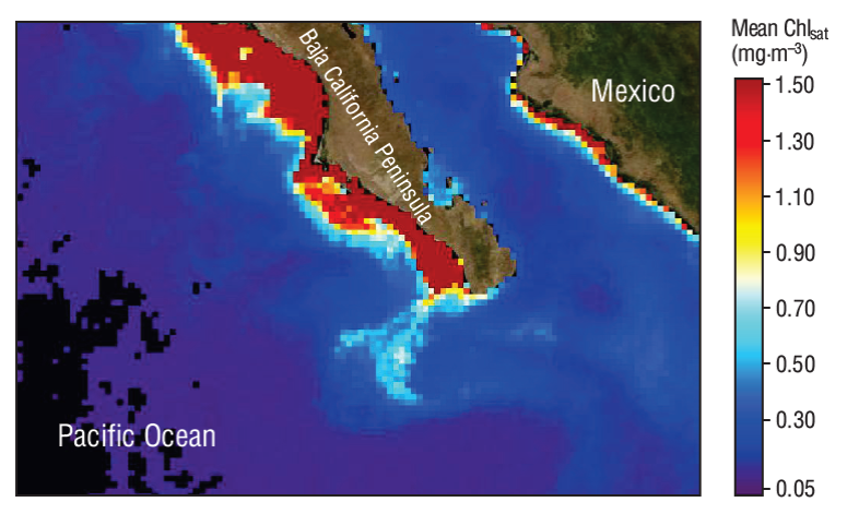
Figure 6 Image showing the California Current flowing away from the Baja California Peninsula and carrying relatively high satellite-derived chlorophyll a concentrations (Chlsat) towards oceanic waters (June 2009).
Satellite imagery shows the spatial distribution of photosynthetic pigments with a rich structure from the coast to hundreds of kilometers offshore, as was reported by Traganza (1985) and many others thereafter. A patchy distribution is caused by a combination of physical, chemical, and biological factors affecting phytoplankton, such as the sequence of upwelling intensification and relaxation (as described by Álvarez-Borrego and Álvarez-Borrego 1982), movements of water masses, mesoscale and sub-mesoscale phenomena, mixing by wind (including storms) or phenomena associated with tides, patchy distribution of nutrients, differential phytoplankton reproduction, and differential grazing (Yentsch 1981). These phenomena were likely the cause for the multiple Chlsat and PP maxima observed in the time series for the coastal quadrants off both capes (Fig. 5). The number of years with multiple PP maxima was lower, compared with that for Chlsat, because the integration with depth in the calculation of PP tends to decrease its variation.
The SST, Chlsat, and PP interannual variations in the inshore zone of our study area could have been caused mainly by the sequence of ENSO events and the Blob. The coldest ENSO phase (La Niña) in our study period occurred in 2011 on both transects, with the lowest SSTs and, in general, the highest Chlsat values, but the 2006, 2008, and 2012 La Niña events were also strong negative ENSO phases (Figs. 3, 4). There are 2 types of El Niño events: the eastern Pacific type (EP), with maximum SST anomalies centered in the region of the eastern equatorial Pacific cold plume; and the central Pacific type (CP), with SST anomalies near the time line (Kao and Yu 2009). The CP type of El Niño has also been referred to as El Niño Modoki (in Japanese meaning similar but different) (Ashok et al. 2007). Propagation of SST anomalies from the Equator to the northeastern Pacific is weaker and less clear in the CP type than in the EP type of El Niño. The EP type of El Niño is characterized by subsurface temperature anomalies that propagate through the Pacific basin; and the CP type of El Niño is more often associated with subsurface temperature anomalies that develop in situ in the central Pacific (Ashok et al. 2007).
The 1982-1983 and the 1997-1998 El Niño events were of the EP type, and it was not until 2015-2016 that another EP type of El Niño occurred, the latter of which impact on the biology of our study area lasted from June 2015 to the end of spring 2016 (Figs. 4, 5). However, El Niño and the Blob were overlapping events and it is not clear if both or only the Blob caused the decrease in Chlsat and PP in the inshore waters of TCSLa and TCSLu throughout most of 2015. After September 2015 El Niño was the main cause for the low phytoplankton biomass observed in our study area. According to Robinson (2016) the recent warming off Baja California occurred in 2 distinct periods. In the first warming period, from May 2014 to April 2015, the SST increase was related to weak coastal winds not associated with El Niño (Robinson 2016). The longest sustained record of negative wind anomalies occurred during this period. Reduced wind stress suggests weakened coastal upwelling. The second warming period occurred from September to December 2015, during strong El Niño conditions (Robinson 2016) (also during 2016 on TCSLu).
Torres-Moye and Alvarez-Borrego (1987) attributed the low phytoplankton biomass they found in coastal waters off northern Baja California in the summer of 1984 to the effect of the 1982-1983 El Niño event. During this event temperatures off Baja California remained high until spring 1984, and macroalgae populations started to recover in autumn 1984 (Hernández-Carmona 1988). The 1997-1998 event did not have the lasting impact the 1982-1984 event had (Ladah et al. 1999). The 1982-1984 event coincided with a warm regime in the North Pacific, while the 1997-1998 event coincided with a cold regime (Newman et al. 2003).
The impact of different ENSO events on phytoplankton and the populations of other organisms is not the same, and it depends, among other things, on the phase of the North Pacific Decadal Oscillation. Kahru and Mitchell (2002) reported that the effects of the 1997-1998 EP type of El Niño were observed as decreased PP starting in mid-1997 and disappearing in 1998 off central and southern California, whereas off southern Baja California, down to the area off CSLa, the effects of this El Niño event became evident later in mid-1998. Using principal component analyses, Herrera-Cervantes et al. (2013) described the interannual SST and Chlsat variability patterns off Punta Eugenia (26-29ºN, 113-116ºW) and suggested that ENSO cycles dominated the SST and Chlsat interannual variations in coastal waters but that variations in deep waters were driven by the intrusion of subarctic water rather than by ENSO cycles.
In the present study, with respect to values from years like 2008, 2011, and 2012, Chlsat and PP decreased by >50% in the TCSLa and TCSLu inshore waters during the Blob in 2014 and during the 2015-2016 EP El Niño. Zaba and Rudnick (2016) reported that, off southern California, the thermocline was depressed and strong stratification lasted from the summer of 2014 through to the 2015-2016 winter. Something similar may have happened in the southernmost part of the CCS, and this would explain the relatively low phytoplankton biomass on TCSLa and TCSLu during this period.
The impact of the El Niño events and the Blob on Chlsat and PP in our study areas is clearly revealed only by the data from the inshore waters and the first season of each year (Figs. 4, 5). Sea surface temperature was higher in the offshore areas of both transects during 2014-2016 than during the other years in our data set (Fig. 3); however, Chlsat and PP during El Niño periods and the Blob did not decrease in the offshore areas. These 2 variables did not decrease because the small-sized phytoplankton typical of oceanic regions is adapted to oligotrophic conditions and has relatively stable populations; most of the Chl variability in rich coastal waters is caused by large-sized phytoplankton (Yentsch and Phinney 1989).
Arroyo-Loranca et al. (2015) analyzed Sea-Viewing Wide Field-of-view Sensor (SeaWIFS) and Aqua-MODIS Chlsat data corresponding to the 1997-2012 period for a transect off Punta Eugenia (off the central part of the peninsula), Baja California Sur, and concluded that, with the exception of the 1997-1998 EP El Niño, ENSO events did not have any significant effect in their study area. Contrary to the findings by Arroyo-Loranca et al. (2015) for the transect off Punta Eugenia, the El Niño events from the twenty-first century did have strong effects on the biology of TCSLa and TCSLu. The 2002-2005 and 2009-2010 El Niño events were of the CP type; in our study, only the 2015-2016 El Niño event was of the EP type (NOAA 2017b). The CP type events tended to occur more often in the twenty-first century (Lee and McPhaden 2010).
The effects of the 2014 Blob event and the 2015-2016 El Niño event were strong off both capes, CSLa and CSLu. While both events had similar effects on TCSLa, the Blob had an apparently stronger effect on TCSLu than El Niño did (Figs. 4, 5). The 2010 CP El Niño was the only one of this type to have a strong impact on TCSLa (Figs. 4, 5). The 2003, 2005, and 2010 CP El Niño events had a strong impact on the biology of TCSLu; their impact was similar to the impact of the Blob in 2014 and the impact of the 2015-2016 EP El Niño (Fig. 4).
According to Lee and McPhaden (2010), the 2009-2010 El Niño was one of the strongest events in the past decades, and this is reflected in the phytoplankton biomass of both transects, TCSLa and TCSLu (Figs. 4, 5). Interannual variations were different off Punta Eugenia, CSLa, and CSLu because of the different coastal dynamics (e.g., upwelling, coastal currents, jets, eddies, and meanders) at each site. The coastal countercurrent shows interannual variations and can affect the physical and biological properties of water off CSLa and CSLu. Satellite altimetry could be used in future studies to better describe these phenomena.
The effects of the ENSO events in the twenty-first century, however, were not drastically strong on TCSLa and TCSLu. Despite the significant decrease in Chlsat and PP, Chlsat values were often >1 mg·m-3 during an ENSO event or the Blob. In other words, phytoplankton biomass did not completely collapse in the southernmost part of the CCS. The Chlsat values decreased to <0.1 mg·m-3 only in 2014 in the TCSLu coastal zone. Putt and Prézelin (1985) reported that, according to their filter fractionation study, over 80% of the chlorophyll-based phytoplankton biomass in the Santa Barbara Channel, California, was <5 µm during El Niño 1982-1983. These authors also reported that the population there as a whole was dominated by cyanobacteria (0.5-1.5 µm), unlike the normal diatom and dinoflagellate dominance in CCS coastal waters (Lara-Lara et al. 1980, Millan-Nuñez et al. 1982). This change in phytoplankton composition during warm events like El Niño and the Blob has drastic effects in the whole CCS coastal ecosystem, including the southernmost portion.
In the coastal zone of the transect off Punta Eugenia, SST minima and Chlsat and PP maxima were ~13 ºC, 26 mg·m-3, and 8.7 g C·m-2·d-1 (Arroyo-Loranca et al. 2015), respectively. These extreme values were ~3 ºC lower than the SST minimum value for TCSLa, and ~6 ºC lower than the SST minimum value for TCSLu. The Punta Eugenia Chlsat maximum was twice the maximum value for TCSLa and 4 times the maximum value for TCSLu, and the Punta Eugenia PP maximum was similar in the case of TCSLa and up to double the maximum value for TCSLu. Mirabal-Gómez et al. (2017) carried out a study similar to ours and analyzed Aqua-MODIS data for the same time period but for a transect off La Jolla, California, and a transect off San Quintín Bay, northwestern Baja California; however, the SST minima in the coastal zone of both their transects were up to 2.5 ºC lower than the SST minima for the TCSLa coastal zone and ~6 ºC lower than the SST minima for TCSLu coastal zone. In general, the lowest Chlsat values were found in the coastal zone off CSLu (this study), the second lowest in the coastal zone off La Jolla, and the highest in the coastal zones off San Quintín Bay, Punta Eugenia, and CSLa. These differences may be due to the fact that coastal upwelling is significantly weaker off La Jolla and CSLu than off the rest of the Baja California Peninsula.
Zuria-Jordán et al. (1995) analyzed Chlsat from the CZCS for a transect that included a section that paralleled the coast of the peninsula (from Point San Hipólito to CSLu). The section of the transect that covered the area off CSLa was very close to the coast, but the section off CSLu was relatively far and covered the oceanic zone. The Chlsat values reported by Zuria-Jordán et al. (1995) for the area near CSLa showed the same seasonality that our values did for the TCSLa coastal zone. These authors reported Chlsat values >8 mg·m-3 for June in the average year for the 1978-1986 period; in our study, Chlsat values for June in the TCSLa climatology were up to 6.5 mg·m-3. Interestingly, data from 2 different sensors showed similar temporal variations for the Chlsat values from the “average years”, not to mention absolute maxima were very close. Zuria-Jordán et al. (1995) reported that the area near CSLa was the richest on their transect. They also reported the strong impact of the 1982-1983 EP El Niño in the coastal area off CSLa, and indicated that the effects lasted until 1985. A comparison of average Chlsat derived from the CZCS (Zuria-Jordán et al. 1995) and average Chlsat derived from Aqua-MODIS for the TCSLa coastal zone (our study) shows that the latter are lower than the former by ~25%. Ramírez-León et al. (2015) compared Gulf of California Chlsat data from the CZCS, SeaWIFS, and Aqua-MODIS and concluded that data from the CZCS tend to grossly overestimate Chlsat.
The PP distribution tends to run parallel to the Chlsat distribution because when calculating PP, Chlsat dominates despite the dependence of PP on SST, photosynthetically active radiation, and day length. This PP behavior was also reported by Álvarez-Molina et al. (2013) for the Gulf of California. PP data show less variability than Chlsat data because PP is integrated for the entire euphotic zone and Chlsat is only an average for the first optical depth (upper 22% of the euphotic zone). When Chlsat is low the euphotic zone is deeper, and integration with depth increases PP.
Our inshore PP values for the first season (February-July) could be overestimated because the VGPM assumes a mixed euphotic zone with homogenous vertical distribution of chlorophyll. In nutrient-rich coastal waters, the chlorophyll maximum is at the surface and values decrease with depth; the assumption that there are no vertical changes in chlorophyll produces PP overestimates. PP values >4 g C·m-2·d-1 are unrealistic and should be taken with caution, considering only the spatial and temporal trends but not the absolute values. Álvarez-Molina et al. (2013) analyzed PP data from the Oregon State University website for the Gulf of California central region and reported that the high values they found for the Guaymas Basin, an area of intense upwelling (PP up to 7.8 g C·m-2·d-1), were possibly overestimated by >50%. Nevertheless, these authors explained that the PP trends were well interpreted, with high values during the upwelling season and very low values in the summer. The variations of our PP data are also well interpreted, with higher values during the upwelling season in February-July than in August-January. According to Kahru and Mitchell (2002), even in the CCS offshore waters (100-300 km from the coast), satellite-derived PP overestimate ship measurements by ~40%. The photosynthetic parameters in the VGPM algorithm for PP taken from the Oregon State University website need to be adjusted for our geographic region, this is an opportunity for future research (Arroyo-Loranca et al. 2015).
The PP data obtained from water samples and 14C incubations are scarce, and it is very difficult to perform comparisons with satellite-derived data. In a strict sense, comparisons between PP data calculated with the VGPM and satellite imagery, and PP estimates from 14C incubations are inappropriate because the 2 data sets have totally different temporal and spatial scales: satellite-derived data are averages for 18 × 18 km2 areas and for a month, while 14C data are instantaneous point measurements (i.e., Balch and Byrne 1994, Kahru and Mitchell 2002). Gaxiola-Castro et al. (2010) reported PP data for the CCS off the Baja California Peninsula, obtained from 14C incubations during 4 cruises per year in the 1998-2007 period. Most of their sampling locations were at >50 km from shore. Gaxiola-Castro et al. (2010) averaged their data set to generate a mean distribution for their study area and reported PP values in milligrams of carbon per square meter per hour. After transforming their average values to grams of carbon per square meter per day, their offshore values were 0.4-0.6 g C·m-2·d-1, which are in agreement with our PP values. Their average values for the inshore region fluctuated between 1.0 and 1.5 g C·m-2·d-1, which are also in agreement with our values considering that most of their sampling sites were not close to shore.

