


 nueva página del texto (beta)
 Inglés (pdf)
 Artículo en XML
 Referencias del artículo
 Enviar artículo por email
 Citado por SciELO
  Similares en
SciELO
Similares en
SciELO 
 Permalink
Introduction
A variety of physical processes in the California Current System (CCS), such as coastal upwelling, jets, and eddies, contribute to the spatial and temporal variations of phytoplankton biomass (chlorophyll, Chl) and production (PP) because they input nutrients to the euphotic zone (Lynn 1967, Pérez-Brunius et al. 2007). In spring there is reduced eddy activity in the CCS. During the rest of the year there are eddies and meanders, although with a predominant southward flux (Durazo et al. 2010). Eutrophic conditions are generally limited to a coastal band, associated with upwelling events, mainly during the months of winter and spring in the south-ern part of the CCS and during late spring and summer in the northern part (Fargion et al. 1993). Lynn and Simpson (1987) defined 3 domains in the CCS: an oceanic domain, a coastal domain, and a transition zone 200-300 km offshore that is parallel to the coast and coincides with the CCS core. Equatorial Water penetrates through the southern limit of the CCS in the form of a subsurface countercurrent near the coast (200 m depth, Lynn and Simpson 1987). At the end of autumn and beginning of winter there is a poleward surface flux in the narrow coastal zone, off the Baja California Peninsula and southern California. This flux is known as the surface coastal countercurrent, commonly known as the Davidson Current (Lynn and Simpson 1987, Reid 1988). There is evidence that this surface and subsurface countercurrents are independent phenomena (Durazo 2015).
The CCS is influenced by El Niño events, which are associated with an increase in sea surface temperature (SST) and a decrease in Chl and PP (Reid 1962, 1988; Putt and Prézelin 1985; Torres-Moye and Álvarez-Borrego 1987; Fargion 1989; Thomas and Strub 1990; Lynn et al. 1998; Kahru and Mitchell 2000, 2002). Events with anomalously low SSTs (La Niña) are associated with relatively high Chl and PP in this area (Kahru and Mitchell 2002). Furthermore, there was a recent anomalous warming of the north Pacific (known by the nickname “Blob”). This phenomenon was detected for the first time in autumn 2013 (Bond et al. 2015), and its effect off southern California and off northern Baja California ended by the end of November 2015 (NOAA 2017a). The Blob was a marine heat wave that produced major disturbances in the California Current ecosystem with great negative economic impacts (Gentemann 2017). It was strongly present off northwestern Baja California (Mexico), with SST values for October 2014 approximately 6 ºC above the maximum temperatures of other years in the period 2008-2014; these values were measured from an anchored buoy in coastal waters off Ensenada, Baja California (Coronado-Álvarez et al. 2017).
Off Ensenada there is a change in the direction of the surface geostrophic flow towards the coast (Reid 1988). This forms the Ensenada Front, which is perpendicular to the coast and extends from 160 to 500 km offshore. In the offshore area, this frontal region separates eutrophic colder waters in the north from the oligotrophic waters in the south, and the frontal structure persists throughout the year (Peláez and McGowan 1986, Gaxiola-Castro and Álvarez-Borrego 1991, Haury et al. 1993). The front is detectable during most of the year but it is strong from the end of March to the beginning of June, and it shows a latitudinal displacement of ~150 km throughout the whole year (Peláez and McGowan 1986). Moreover, the position of the front is affected by El Niño/Southern Oscillation (ENSO) events (Santamaría-del-Ángel et al. 2002). When this surface geostrophic flux reaches the coast, it splits into two: one flux flows northward into the cyclonic circulation of the Southern California Bight and the other flows southward (Peláez and McGowan 1986). The latter flux turns offshore off San Quintín Bay, similar to the offshore flux off Point Conception, California (USA). These fluxes that veer from the coast intensify coastal upwelling (Álvarez-Borrego 2004).
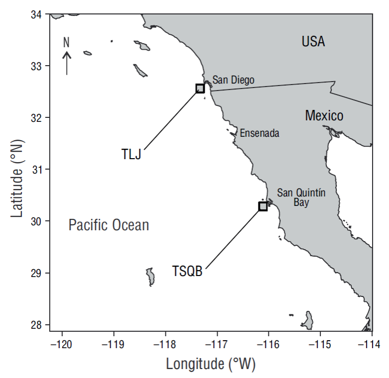
The main objective of this work was to characterize the spatial and temporal variations of Chl and PP off La Jolla, California, and off San Quintín Bay, Baja California, (Fig. 1) to compare 2 different oceanographic conditions given their geographic positions with respect to the Ensenada Front. The study used data generated by a satellite sensor, covering the seasonal and interannual scales; emphasis was made on the effect of physical processes such as upwelling, El Niño, and the Blob.
Materials and methods
Study areas
The area off La Jolla is inside the cyclonic eddy of the Southern California Bight (SCB). In the SCB there are relatively weak, upwelling-favorable winds compared with other regions along the CCS, and the maximum wind stress axis is further away from the coastline; wind speeds in the SCB are lower than wind speeds 140 km offshore by a factor of 2 or more (Dorman 1982, Winant and Dorman 1997). There is a strong poleward flow in the coastal zone, mainly in autumn and winter. This poleward flow weakens in spring. South of Point Conception, this flow appears as a large cyclonic eddy over the SCB offshore banks (Lynn and Simpson 1987). The atmospheric flow separates from the coast near Point Conception, producing a large wind stress curl with an average Ekman pumping of 4 m·d-1, and with strong persistent winds this pumping may reach 20 m·d-1 (Münchow 2000).
Upper layer Chl, both measured from water samples and by remote sensing, exhibits significant seasonal variation in the SCB, and it is highest in mid and late winter and lowest in summer (Eppley et al. 1985, Michaelsen et al. 1988). Integrated (0-150 m) Chl in the SCB, within CalCOFI (California Cooperative Oceanic Fisheries Investigations) line 90, showed a weak seasonal signal, with the April-May mean well above the overall mean; but the monthly bight-wide, space aver-aged, integrated Chl, and the surface, space averaged Chl did not show a seasonal pattern (Fargion et al. 1993). There is a clear onshore-offshore gradient in all seasons for surface Chl to be higher in the coastal zone than in the offshore zone of the SCB (Fargion et al. 1993).
The area off San Quintín Bay is characterized by high Chl and PP because of intense upwelling (Lara-Lara et al. 1980, Álvarez-Borrego and Álvarez-Borrego 1982, Millán-Núñez et al. 1982). In the open ocean, near the mouth of San Quintín Bay, upwelling events occur from April to October, with the most intense during spring and summer as a result of the dominance of northwesterly winds (Álvarez-Borrego and Álvarez-Borrego 1982) and the coastal circulation induced by the Ensenada Front (Álvarez-Borrego 2004). Off San Quintín Bay circulation has 2 components: one is parallel to the coast and has an equatorward direction, and the other is offshore to compensate the onshore component of transport at the Ensenada Front (Álvarez-Borrego 2004).
Satellite data
Monthly composites of SST and Chlsat from the Moderate Resolution Imaging Spectroradiometer aboard the Aqua satellite (Aqua-MODIS) for the July 2002-December 2016 period were used to generate the time series. These composites were obtained from the National Aeronautics and Space Administration (NASA) Ocean Color web page (NASA 2017), with level 3 and 9 × 9 km2 pixel size. The SST data are from day measurements with 11 μm radiation. All PP imagery were obtained from the Ocean Net Primary Productivity website of the Oregon State University (OSU 2017). Images were downloaded in Hierarchical Data Format (.hdr format). Phytoplankton production is given as a standard product already calculated using the Behrenfeld and Falkowsky (1997) vertically generalized productivity model (VGPM). The VGPM is a non-spectral model with homogeneous vertical distribution of Chl and with vertically integrated PP. Pixel size for PP was 18 × 18 km2. Satellite imagery was processed with software from the NASA Ocean Color web page (NASA 2017).
Two 250-km long transects perpendicular to the coast (Fig. 1), one off La Jolla (TLJ) and the other off San Quintín Bay (TSQB), were sampled from the monthly composites to describe the spatial and temporal variations of SST, Chlsat, and PP. We described a first approximation to the climatology of the region based on an “average year” for each variable and for each transect. This climatology consisted in averaging data for the Januaries of all years, then data for all Februaries, and so on for all months. In order to describe the temporal variation in more detail, we generated time series with the monthly averages of the variables from an 18 × 18 km2 coastal quadrant off La Jolla (centered at 31.66ºN, 116.99ºW) and another one off San Quintín Bay (centered at 30.66ºN, 116.33ºW) (Fig. 1), from July 2002 through December 2016. Matlab 2014b was used for the spectral analysis of the time series in order to characterize the relative magnitude of the different components of variation.
STATISTICA v.7.0.2 software was used for the statistical analysis. Chlsat distributions were not normal. Each year was divided into 2 seasons and each transect into 2 zones (one inshore zone and one offshore zone). Thus, non-parametric Mann-Whitney tests were performed to explore Chlsat differences between the 2 seasons for each zone on each transect, between the 2 zones on each transect, and between transects. Matlab 2014b was used to build Hovmöller diagrams with SST and Chlsat data from all years.
The Multivariate El Niño Index (NOAA 2017b) was used to distinguish between El Niño, La Niña, and “normal” conditions.
Results
In general, the average year showed very clear variations in Chlsat and PP between inshore and offshore areas, with higher values in the zone near the coast. On the other hand, SST showed a different spatial variation, with lower values near the coast than offshore on both transects but mainly on TSQB. On TLJ the SST gradient was inverted in July and August, with higher values near the coast than offshore. In June SST variations were irregular for both transects (Fig. 2).

Figure 2 Climatology of the 3 variables for the transect off La Jolla (TLJ) (left panels) and the transect off San Quintín Bay (TSQB) (right panels).
Throughout the average year, the SST differences from near the coast to further offshore ranged from a few tenths of a degree to ~5.7 ºC on TLJ. The maximum SST value (20.8 ºC) for this transect occurred in September at ~50 km from shore, whereas the minima (~15.2 ºC) occurred in January, February, and March near the coast. On this transect, SST showed almost no spatial variations in May, fluctuating a few tenths of a degree around 17 ºC. For TSQB the SST spatial differences ranged from a few tenths of a degree to ~6.7 ºC throughout the average year. The maximum SST value (~21.2 ºC) for this transect also occurred in September, and minima (~14.7 ºC) occurred in February, March, and April.
Taking into account the spatial distribution of Chlsat for the average year, we may consider the inshore zone to extend seaward from the coast to ~50 km for both transects (Fig. 2) and the offshore zone to extend from ~50 km and beyond. In general, when taking the 2-mg·m-3 value as a criterion to separate eutrophic waters from mesotrophic waters in the coastal zone, the Chlsat climatology for both transects showed 2 seasons with different biological conditions. The first season for TLJ was from March to June, with the highest Chlsat value (3.2 mg·m-3) occurring in April, and the first season for TSQB was from February to June, with the maximum Chlsat value (11.9 mg·m-3) occurring in March. During the second season, maxima Chlsat in the inshore zone were 1.3 mg·m-3 (August) for TLJ and 1.5 mg·m-3 (January) for TSQB. Throughout the average year the lowest value for both transects was ~0.1 mg·m-3 in the furthest offshore area (200 to 250 km).
The PP plots for the average year were very similar to the Chlsat plots, with high values near the coast decreasing with distance from the coast (Fig. 2). In the coastal zone, the first season maxima occurred in April (4.9 g C·m-2·d-1 for TLJ and 4.3 g C·m-2·d-1 for TSQB) and those for the second season occurred in July (3.0 g C·m-2·d-1 for TLJ and 1.6 g C·m-2·d-1 for TSQB). For TLJ, PP minima were ~0.5 g C·m-2·d-1 in the first season and ~0.4 g C·m-2·d-1 in the second season, and both values were detected in the farthest offshore area. For TSQB, PP minima in both seasons were 0.4 g C·m-2·d-1 and occurred also in the farthest offshore area.
The month-to-month SST variation showed clear seasonal and interannual components for both transects. The SST spatial distribution on TLJ was irregular, with several minima and maxima in most months, although with a slight tendency to show the lowest values near the coast. On TSQB the SST spatial distribution was regular and monotonic, with lower values near the coast than offshore. During the study period the SST range for TLJ was 13.6-24.0 ºC in the inshore zone and 11.9-23.6 ºC in the offshore zone; for TSQB the range was 13.2-25.1 ºC in the inshore zone and 12.0-25.0 ºC in the offshore zone. The SST differences between both transects, for every month, were similar for both zones, exceptionally up to 1.2 ºC for the inshore zone and up to 2.3 ºC for the offshore zone, often with higher values in the TLJ inshore zone than in the TSQB inshore zone. Along both transects, SST minima occurred in winter-spring and SST maxima occurred in summer and the beginning of autumn (Table 1).
Table 1 Sea surface temperature (SST, ºC) minima and maxima, and the month on which they occurred, for the inshore (0 to 50 km) and offshore zones on the transect off La Jolla (TLJ) and the transect off San Quintín Bay (TSQB) in each year.
| TLJ Inshore | 2002 | 2003 | 2004 | 2005 | 2006 | 2007 | 2008 | 2009 | 2010 | 2011 | 2012 | 2013 | 2014 | 2015 | 2016 |
| Min. SST | 16.2 | 14.9 | 14.8 | 15.0 | 14.0 | 14.3 | 13.6 | 14.9 | 15.2 | 14.2 | 14.2 | 14.2 | 15.8 | 17.0 | 16.2 |
| Dec | Apr | Feb | Dec | Mar | Dec | Apr | Feb | Dec | Mar | Mar | Feb | Apr | Jan | Feb | |
| Max. SST | 19.6 | 21.7 | 21.8 | 21.2 | 21.7 | 21.8 | 21.4 | 21.6 | 19.2 | 19.6 | 21.9 | 21.3 | 22.7 | 24.0 | 22.5 |
| Jul | Sep | Sep | Aug | Jul | Aug | Aug | Sep | Oct | Sep | Sep | Sep | Sep | Oct | Aug | |
| TLJ Offshore | 2002 | 2003 | 2004 | 2005 | 2006 | 2007 | 2008 | 2009 | 2010 | 2011 | 2012 | 2013 | 2014 | 2015 | 2016 |
| Min. SST | 16.3 | 15.7 | 15.2 | 15.7 | 15.0 | 14.9 | 13.0 | 15.2 | 11.9 | 14.4 | 14.8 | 14.7 | 15.8 | 17.5 | 16.4 |
| Dec | Jun | Feb | Feb | Mar | Jan | Jun | May | Jun | Feb | Mar | Feb | Feb | Jan | Jan | |
| Max. SST | 19.8 | 21.6 | 21.8 | 21.1 | 21.8 | 21.1 | 20.9 | 21.6 | 19.2 | 20.3 | 22.0 | 21.2 | 22.9 | 23.6 | 21.7 |
| Sep | Sep | Sep | Aug | Aug | Aug | Aug | Sep | Aug | Sep | Sep | Sep | Sep | Sep | Aug | |
| TSQB Inshore | 2002 | 2003 | 2004 | 2005 | 2006 | 2007 | 2008 | 2009 | 2010 | 2011 | 2012 | 2013 | 2014 | 2015 | 2016 |
| Min. SST | 15.8 | 13.6 | 14.5 | 14.6 | 13.2 | 13.6 | 13.7 | 14.0 | 14.2 | 13.2 | 13.6 | 14.1 | 15.2 | 16.4 | 16.0 |
| Dec | May | Feb | Apr | Mar | Apr | Feb | Mar | Dec | Mar | Mar | Feb | Apr | May | Mar | |
| Max. SST | 19.5 | 21.7 | 21.8 | 20.8 | 22.0 | 21.4 | 20.7 | 21.7 | 18.8 | 20.2 | 22.2 | 21.1 | 22.8 | 25.1 | 22 |
| Sep | Sep | Sep | Aug | Sep | Aug | Oct | Sep | Sep | Sep | Sep | Aug | Sep | Jul | Sep | |
| TSQB Offshore | 2002 | 2003 | 2004 | 2005 | 2006 | 2007 | 2008 | 2009 | 2010 | 2011 | 2012 | 2013 | 2014 | 2015 | 2016 |
| Min. SST | 16.8 | 13.4 | 15.2 | 16 | 14.4 | 15.2 | 14.6 | 14.7 | 12.0 | 5.9 | 15.1 | 14.8 | 16.3 | 17.9 | 16.9 |
| Dec | Jun | Feb | Feb | Mar | Apr | Feb | Mayo | Jun | Mar | Mar | Feb | Feb | Feb | Jan | |
| Max. SST | 20.4 | 21.8 | 22.1 | 21.5 | 22.1 | 21.1 | 21.2 | 21.9 | 19.1 | 20.9 | 22.5 | 21.5 | 23.3 | 25.0 | 22.1 |
| Sep | Sep | Sep | Aug | Sep | Sep | Oct | Sep | Aug | Sep | Sep | Sep | Oct | Jul | Sep | |
Hovmöller diagrams showed that on TLJ, even though minimum SST was detected in offshore waters in June 2010 (Table 1), waters along the entire transect were colder in the first seasons of 2007-2009 and 2011-2012 than in the other years of our study period. Conversely, 2015 showed higher SSTs than the rest of the years, although 2014 and 2016 were also relatively warm years (Fig. 3). A similar situation was observed for TSQB, with 2015 as the warmest year. Also on TSQB, there was a clear SST gradient with colder waters in the coastal zone than offshore during “normal” and warm years. This gradient was not clear during the cold 2007-2012 period. During the second season, waters were relatively warm along the entire extension of both transects (Fig. 3). Thus, there was a clear SST seasonal signal throughout the transects.

Figure 3 Hovmöller diagrams for sea surface temperature (SST) along the transect off La Jolla (upper panel) and the transect off San Quintín Bay (lower panel).
On TLJ the SST gradient was inverted in summer, with higher inshore than offshore values, as mentioned above. But this inversion changed from year to year, often taking place between June and August, and in some years it began in May and ended until September. During this gradient reversal, SST differences between inshore warm waters and offshore waters with lower SST ranged from ~0.7 ºC (in most cases) to ~2.5 ºC.
In the inshore zone of both transects there were Chlsat and PP variations with clear seasonal and interannual components (Tables 2, 3). In the month-to-month variation, Chlsat and PP values were relatively high (≥1.0 mg·m-3 and ≥1.0 g C·m-2·d-1, respectively) in the TLJ inshore zone during spring and summer, although high values were occasionally observed further from shore (70-160 km). Values >1.0 mg·m-3 and >1.0 g C·m-2·d-1 were frequently observed for autumn and winter. In the TSQB inshore zone, the month-to-month Chlsat and PP variations often presented relatively high values (≥1.0 mg·m-3 and ≥1.0 g C·m-2·d-1, respectively) in winter, spring, and summer.
Table 2 Phytoplankton biomass obtained from satellite imagery (Chlsat, mg·m-3) and primary production (PP, g C·m-2·d-1) minima and maxima for the inshore (0 to 50 km) and furthest offshore (~250 km) zones on the transect off La Jolla (TLJ) in each year.
| TLJ Inshore | 2002 | 2003 | 2004 | 2005 | 2006 | 2007 | 2008 | 2009 | 2010 | 2011 | 2012 | 2013 | 2014 | 2015 | 2016 |
| Min. Chlsat | 0.2 | 0.2 | 0.1 | 0.1 | 0.1 | 0.1 | 0.1 | 0.1 | 0.2 | 0.2 | 0.1 | 0.1 | 0.1 | 0.1 | 0.1 |
| Jul | Feb | Aug | Mar | Jul | Aug | Aug | Aug | May | Aug | Aug | Aug | Oct | Aug | Mar | |
| Min. PP | 0.6 | 0.5 | 0.5 | 0.5 | 0.7 | 0.8 | 0.7 | 0.6 | 0.8 | 0.8 | 0.6 | 0.5 | 0.4 | 0.4 | 0.4 |
| Dec | Jan | Feb | Feb | Feb | Aug | Nov | Oct | Dec | Dec | Aug | Dec | Dec | Aug | Oct | |
| Max. Chlsat | 1.4 | 12.0 | 2.9 | 7.5 | 5.1 | 4.4 | 9.7 | 3.6 | 3.2 | 6.5 | 9.6 | 3.1 | 2.5 | 2.3 | 1.5 |
| Aug | May | Jun | Aug | Mar | May | Apr | Jun | Aug | Mar | Mar | Apr | Apr | Jun | Jun | |
| Max. PP | 3.5 | 5.5 | 5.4 | 8.6 | 6.3 | 5.9 | 7.5 | 7.5 | 4.7 | 4.4 | 5.3 | 4.0 | 3.1 | 4.9 | 3.4 |
| Jul | May | Apr | Jun | Apr | Apr | Apr | Jun | Mar | Jun | Mar | Apr | May | Apr | May | |
| TLJ Offshore | 2002 | 2003 | 2004 | 2005 | 2006 | 2007 | 2008 | 2009 | 2010 | 2011 | 2012 | 2013 | 2014 | 2015 | 2016 |
| Min. Chlsat | <0.1 | <0.1 | <0.1 | <0.1 | <0.1 | <0.1 | <0.1 | <0.1 | 0.1 | <0.1 | 0.1 | <0.1 | <0.1 | 0.1 | 0.1 |
| Sep | Oct | Jul | Jul | Jul | Aug | Aug | Jul | Nov | May | Sep | Jun | Sep | Oct | May | |
| Min. PP | 0.3 | 0.3 | 0.3 | 0.3 | 0.3 | 0.3 | 0.3 | 0.3 | 0.3 | 0.3 | 0.3 | 0.3 | 0.2 | 0.3 | 0.4 |
| Sep | Feb | Nov | Mar | Feb | Sep | Aug | Jul | Nov | Sep | Sep | Jun | Dec | Oct | Oct | |
| Max. Chlsat | 0.6 | 0.5 | 0.4 | 4.2 | 4.6 | 0.7 | 1.9 | 0.7 | 1.7 | 1.1 | 0.8 | 0.5 | 0.2 | 0.5 | 0.4 |
| Aug | Sep | Feb | Jul | May | Feb | Apr | Feb | Dec | Jan | May | Feb | Feb | May | Jun | |
| Max. PP | 1.2 | 2.8 | 0.8 | 2.9 | 2.1 | 1.4 | 1.6 | 1.3 | 1.4 | 1.6 | 1.5 | 1.4 | 0.9 | 1.0 | 0.9 |
| Aug | May | Jun | Jul | May | Apr | Apr | Jun | Jul | Apr | May | Jul | May | May | May |
Table 3 Phytoplankton biomass obtained from satellite imagery (Chlsat, mg·m-3) and primary production (PP, g C·m-2·d-1) minima and maxima for the inshore (0 to 50 km) and furthest offshore (~250 km) zones on the transect off San Quintín Bay (TSQB) in each year.
| TSQB Inshore | 2002 | 2003 | 2004 | 2005 | 2006 | 2007 | 2008 | 2009 | 2010 | 2011 | 2012 | 2013 | 2014 | 2015 | 2016 |
| Min. Chlsat | 0.2 | 0.1 | 0.1 | 0.2 | 0.1 | 0.1 | 0.1 | 0.1 | 0.2 | 0.1 | 0.1 | 0.1 | 0.1 | 0.1 | 0.1 |
| Nov | Sep | Jul | Mar | Aug | Sep | Sep | Sep | Oct | Sep | Jul | Jul | Jun | Jul | Apr | |
| Min. PP | 0.5 | 0.4 | 0.4 | 0.5 | 0.5 | 0.6 | 0.4 | 0.4 | 0.5 | 0.5 | 0.4 | 0.5 | 0.3 | 0.4 | 0.5 |
| Nov | Nov | Jan | Feb | Sep | Jan | Oct | Sep | Oct | Nov | Sep | Nov | Nov | Jan | Oct | |
| Max. Chlsat | 1.7 | 15.8 | 6.0 | 22.5 | 9.7 | 12.1 | 16.8 | 16.0 | 15.6 | 38.6 | 20.5 | 5.7 | 9.6 | 6.3 | 7.5 |
| Nov | May | Apr | Apr | Apr | Apr | Mar | Mar | Apr | Mar | Mar | Mar | Mar | Apr | Apr | |
| Max. PP | 1.8 | 6.1 | 2.9 | 6.0 | 4.5 | 6.4 | 6.1 | 4.2 | 6.5 | 5.6 | 4.9 | 4.1 | 2.5 | 3.8 | 4.5 |
| Sep | May | Apr | Apr | Apr | Apr | Mar | Apr | May | Mar | Mar | Apr | Apr | Apr | May | |
| TSQB Offshore | 2002 | 2003 | 2004 | 2005 | 2006 | 2007 | 2008 | 2009 | 2010 | 2011 | 2012 | 2013 | 2014 | 2015 | 2016 |
| Min. Chlsat | <0.1 | <0.1 | <0.1 | <0.1 | <0.1 | <0.1 | <0.1 | <0.1 | <0.1 | <0.1 | <0.1 | <0.1 | <0.1 | 0.1 | <0.1 |
| Oct | Aug | Apr | Jul | Jun | Sep | Sep | Sep | Aug | May | May | May | Jun | Jul | Jul | |
| Min. PP | 0.3 | 0.3 | 0.3 | 0.3 | 0.3 | 0.3 | 0.4 | 0.2 | 0.3 | 0.3 | 0.3 | 0.3 | 0.2 | 0.3 | 0.3 |
| Oct | Oct | Feb | Mar | Apr | May | Mar | Sep | Oct | May | Aug | Dec | Dec | Jan | Aug | |
| Max. Chlsat | 0.5 | 6.1 | 0.7 | 0.6 | 2.4 | 0.6 | 1.8 | 1.8 | 2.5 | 0.5 | 0.7 | 1.2 | 0.2 | 0.2 | 0.3 |
| Oct | May | Sep | Jul | Mar | Jun | Mar | May | May | May | May | Mar | Apr | Dec | Jun | |
| Max. PP | 1.0 | 3.1 | 1.4 | 2.2 | 2.0 | 1.7 | 1.6 | 2.2 | 2.2 | 1.8 | 1.5 | 1.2 | 0.6 | 0.6 | 0.8 |
| Sep | May | Apr | Jul | Mar | Jun | Apr | May | May | Jun | May | Apr | Apr | Aug | Jun |
Inshore Chlsat maxima were higher on TSQB (up to 38.6 mg·m-3) than on TLJ (up to 12.0 mg·m-3), and minima for both transects were similar. On TLJ, sometimes maximum Chlsat was not near the coast but between 30 and 150 km. On TSQB, maximum Chlsat was, on a few occasions, on the second pixel near the coast. In the TSQB inshore zone, Chlsat showed exceptionally high values in 2005, 2011, and 2012. Offshore Chlsat maxima on TLJ were relatively high (up to 4.6 mg·m-3), while those on TSQB were generally low (0.7 mg·m-3) but exceptionally as high as 6.1 mg·m-3. The PP plots and the Chlsat plots behaved very similar, although PP values in inshore waters were greater on TLJ (up to 8.6 g C·m-2·d-1) than on TSQB (up to 6.5 g C·m-2·d-1) (Tables 2, 3).
Hovmöller diagrams for Chlsat on both transects showed greater spatial and temporal variations than those for SST (Figs. 3 , 4). Seasonal and interannual variations were evident for Chlsat and SST but with greater contrast for Chlsat than for SST. Chlsat was higher in the TSQB inshore zone than those in the TLJ inshore zone. In the Chlsat diagram for TLJ, values were relatively high offshore, mainly in 2005, 2006, and 2011. In 2005 values were >4 mg·m-3 in patches from the inshore zone to ~140 km from the coast; in 2011 values were ~2 mg·m-3 in patches from the inshore zone to ~200 km from the coast (Fig. 4). There were also relatively high Chlsat values (~2 mg·m-3) in TSQB waters >100 km offshore in 2008, 2009, and 2013. In the TLJ inshore zone Chlsat values were very low in 2004, 2014, 2015, and 2016, but in the TSQB inshore zone Chlsat values were low only in 2004 (Fig. 4).

Figure 4 Hovmöller diagrams for Phytoplankton biomass (Chlsat) along the transect off La Jolla (upper panel) and the transect off San Quintín Bay (lower panel).
Results from the Mann-Whitney tests comparing Chlsat between the 2 seasons, the 2 zones, and the 2 transects indicate significant differences in all cases, with the exception of Chlsat values for the inshore zones of both transects in the second season, which were not significantly different between transects (Table 4). These tests and the visualization of the data indicate that, in general, Chlsat values were significantly higher in the first season than in the second season in both zones of both transects; that Chlsat values were significantly higher in the inshore zones than in the offshore zones of both transects in both seasons; and that Chlsat values were significantly higher in the inshore zone of TSQB than in the inshore zone of TLJ in the first season. In the offshore zone, Chlsat values were significantly higher on TLJ than on TSQB in both seasons.
Table 4 Results of Mann-Whitney tests comparing phytoplankton biomass (Chlsat) pairs of data sets as indicated (transect off La Jolla [TLJ], transect off San Quintín Bay [TSQB], coastal zone [IN], off-shore zone [OFF]). Significant differences are marked in bold.
| TLJ | First season IN vs second IN | n = 570 | P < 0.001 |
| First season OFF vs second OFF | n = 2,220 | P < 0.045 | |
| TSQB | First season IN vs second IN | n = 574 | P < 0.001 |
| First season OFF vs second OFF | n = 2,213 | P < 0.001 | |
| TLJ | First season IN vs OFF | n = 1,118 | P < 0.001 |
| Second season IN vs OFF | n = 1,672 | P < 0.001 | |
| TSQB | First season IN vs OFF | n = 1,118 | P < 0.001 |
| Second season IN vs OFF | n = 1,665 | P < 0.001 | |
| IN | First season TLJ vs TSQB | n = 472 | P < 0.001 |
| Second season TLJ vs TSQB | n = 672 | P < 0.822 | |
| OFF | First season TLJ vs TSQB | n = 1,764 | P < 0.001 |
| Second season TLJ vs TSQB | n = 2,665 | P < 0.001 |
The time series for the coastal quadrants off La Jolla (QLJ) and off San Quintín Bay (QSQB) showed clear seasonal and interannual variations, with higher variance in the annual cycle (Fig. 5). In both quadrants, maxima SST (23.9 ºC) and the highest yearly SST minima (~17.5 ºC) occurred in 2015. The largest seasonal SST difference for QLJ was ~7.8 ºC and that for QSQB was ~8.1 ºC, both occurring in 2006. The largest differences between maxima of consecutive years were 2.5 ºC for QLJ and 2.9 ºC for QSQB, both between 2009 and 2010. The Chlsat time series for QSQB, where each number is an average for 4 pixels, showed no exceptionally high values for 2005, 2011, and 2012 such as those observed for the transect (Fig. 5, Table 2). In this time series the highest values were up to 11.6 mg·m-3 and occurred in 2003, 2007, and 2008. The highest Chlsat values for QLJ were recorded in 2003, 2008, and 2012, and they were up to 9.5 mg·m-3. The lowest Chlsat values for QLJ were recorded in 2014, 2015, and 2016, and the lowest for QSQB were recorded in 2004 and 2015. The largest seasonal Chlsat difference for QLJ was ~7.9 mg·m -3, in 2008, and that for QSQB was ~11.2 mg·m-3, in 2003. The largest difference between Chlsat maxima for consecutive years was 6.1 mg·m-3, between 2008 and 2009, for QLJ and 10.6 mg·m-3, between 2003 and 2004, for QSQB. In the time series for QLJ and QSQB, PP values were parallel to those of Chlsat but showed no extreme minima (Fig. 5).

Figure 5 Time series of sea surface temperature (SST) off La Jolla (a), SST off San Quintín Bay (b), phytoplankton biomass (Chlsat) and primary production (PP) off La Jolla (c), and Chlsat and PP off San Quintín Bay (d) in the 18 × 18 km2 coastal quadrants.
The time series spectral analysis confirms that most of the variance occurred in the annual period (not illustrated). Spectral variances for the SST time series were very similar for both quadrants. In the case of Chlsat and PP, however, spectral variances for the QSQB time series were greater than those for the QLJ time series. The SST time series spectral variance for both quadrants showed very small intra-annual variation, while those for Chlsat and PP showed peaks of spectral variance at different intra-annual frequencies (semiannual and other frequencies). Spectral analysis did not clearly show the interannual components of variance, possibly because our time series were very short (not illustrated).
Discussion
In the inshore zone of both transects, the seasonal cycle of SST, Chlsat, and PP is related to the dynamics of the CCS. The California Current flux and coastal upwelling intensify in spring and the beginning of summer, promoting a strong seasonal biological signal, as described by Espinosa-Carreón et al. (2004). Lynn et al. (1982) indicated that a late spring-early summer phytoplankton bloom in the California Current occurs because that is when the stability maximum shoals and intensifies inshore. At the end of autumn and beginning of winter the California Current flux and coastal upwelling are weak, and there is a surface countercurrent near the coast (Lynn and Simpson 1987, Durazo et al. 2010). This winter coastal surface countercurrent clearly produces higher SST and lower Chlsat and PP values than the values observed for spring and summer (Figs. 2-4). As Arroyo-Loranca et al. (2015) indicated, the Coriolis Effect causes the surface countercurrent to inhibit coastal upwelling because it tends to accumulate water near the coast. However, our data show that in the weak upwelling period (second season) the Chlsat values from the inshore zones of both transects often reached >1 mg·m-3 (Figs. 2, 4), which indicates mesotrophic conditions. Thus, as Fargion (1989) indicated, the seasonal variation does not produce an extreme inshore oligotrophic situation during winter. As a comparison, Santamaría-del-Ángel et al. (1999) used data from the Coastal Zone Color Scanner for the Gulf of California to conclude that during the season with no upwelling, Chlsat collapses to <<0.1 mg·m-3. In the furthest offshore area there was no clear biological seasonal signal for either transect (Fig. 4), as was reported by Fargion et al. (1993).
Kahru and Mitchell (2000) proposed dividing the CCS surface waters into an inshore eutrophic zone, an intermediate mesotrophic zone, and an offshore oligotrophic zone, under the criteria that eutrophic means Chlsat is >1.0 mg·m-3 and mesotrophic means Chlsat is between 0.25 and 1.0 mg·m-3. Based on Chlsat data from the inshore zones of both transects, we divided the year into 2 seasons considering the values >2.0 mg·m-3 as indicative of eutrophic conditions, and values <2.0 mg·m-3 as indicative of mesotrophic conditions. We considered this criteria to be more appropriate because the inshore zones of both transects showed relatively high Chlsat values even during the weak upwelling season.
The northward coastal flux in the SCB cyclonic eddy caused upwelling events in spring and the beginning of summer to be less intense on TLJ than on TSQB. Also, the offshore component of circulation off San Quintín Bay may intensify upwelling events on TSQB, as suggested by Álvarez-Borrego (2004) (see also the plume with relatively high Chlsat values going offshore from the coastal zone off San Quintín Bay in Fig. 6). These upwelling events lead to higher Chlsat values on TSQB compared with those on TLJ (Figs. 2, 4; Table 2). This also explains the lower seasonal component of variance for Chlsat and PP on TLJ than on TSQB in the spectral analysis (not illustrated). According to Eppley et al. (1979), surface nitrate concentration is very low in southern California coastal waters, except during short periods of strong upwelling. However, PP values on TLJ were often higher than those on TSQB (Table 3) because nitrate concentration off southern California increases with depth in the euphotic zone (Eppley et al. 1979) and because Chlsat was lower and the euphotic zone was deeper on TLJ than on TSQB; a deeper euphotic zone increases PP, as shown by Lara-Lara et al. (1984) with in situ Chl and PP data from 14C incubations in the Gulf of California. The relatively high Chlsat values in the TLJ offshore zone, up to ~200 km from the coast in years like 2005, 2006, and 2011(Fig. 4), were caused by upwelling jets coming from Point Conception and by Ekman pumping, as described by Münchow (2000) (see Fig. 6).

Figure 6 Example of an image showing plumes of relatively high phytoplankton biomass (Chlsat) flowing from Point Conception into the Southern California Bight (June 2005). Note the small plume flowing offshore from San Quintín Bay. The white areas are either land or areas lacking Chlsat data because of persistent clouds.
Interannual variations in SST, Chlsat, and PP in the inshore zone of both transects were somewhat irregular (Fig. 4). This and the presence of several SST, Chlsat, and PP minima and maxima along the transects during certain months (not illustrated), with no clear temporal pattern of variation, might indicate the influence of mesoscale phenomena. Strub et al. (1991) and Soto-Mardones et al. (2004) reported the presence of cyclonic and anticyclonic eddies off Baja California. Durazo et al. (2005) reported eddies and meanders in the CCS region off the northern and central parts of the peninsula. These mesoscale phenomena affect biological production in the study area, mainly along TLJ (Fig. 4) (Henson and Thomas 2007a, b).
The inshore SST, Chlsat, and PP interannual variations may have been caused mainly by the sequence of ENSO events and the Blob. Arroyo-Loranca et al. (2015) used Chlsat Sea-viewing Wide-Field-of-view Sensor (SeaWIFS) and Aqua-MODIS data for a transect off Punta Eugenia (TPE) (27º38 N), Baja California Sur, and concluded that, with the exception of the 1997-1998 El Niño, which was of the eastern Pacific (EP) type, Chlsat data did not show any significant effect of El Niño events on their study area in the 1997-2012 period. However, the twenty-first century El Niño events have had significant effects on the biology of our study area. The 1982-1983 and the 1997-1998 El Niño events were of the EP type; in the twenty-first century, it was not until 2015-2016 that there was another EP type of El Niño. The 2002-2003, 2004-2005, and 2009-2010 El Niño events were of the central Pacific (CP) type. The CP type events have occurred more often in the twenty-first century (Lee and McPhaden 2010). The 2014 Blob and the 2015-2016 El Niño had a very strong effect on the TLJ inshore zone, with low Chlsat values in the first season during 3 consecutive years; however, the impacts of these 2 events were not as strong on TSQB, since very low Chlsat values were found only in 2015 (Figs. 4, 5). On the other hand, the 2004 CP type of El Niño had the same strong impact on both transects, TSQB and TLJ (Fig. 5), with the effect on Chlsat as severe as that from the 2015 overlap of the Blob and the EP type of El Niño. The impact of ENSO events and other “anomalous warmings” is different along the different coastal areas of the CCS because of coastal dynamics, such as circulation, jets, eddies and meanders, and physiography (capes, islands). Using underwater gliders, Zaba and Rudnick (2016) found that off southern California, the thermocline was depressed and stratification was high from the summer of 2014 to the winter of 2015-2016. This may explain the very low Chlsat values off La Jolla during 2014-2016. In addition, ENSO and other warming events may change significantly from location to location along the different coastal areas of the CCS, causing different biological effects, and this geographic variation raises an opportunity for future research. Our time series are too short for the spectral analysis to show clear interannual components of variance, but variations were present at periods larger than 2 years (not illustrated).
Since there was a time overlap of El Niño and the Blob, it is not clear if both events or only the Blob caused the decrease in Chlsat and PP in the inshore waters of TLJ and TSQB throughout most of 2015. After September 2015 the effect of El Niño was the main cause for the low Chlsat values in our study area. According to Robinson (2016), recent warming off Baja California occurred during 2 distinct periods: the first period occurred from May 2014 to April 2015, when SST increased because of weak coastal winds not associated with El Niño, the longest sustained record of negative wind anomalies occurred, and reduced wind stress suggested weak coastal upwelling; and the second period occurred from September to December 2015, when there were strong El Niño conditions (and clearly also during 2016 on TLJ).
The 2009-2010 El Niño was one of the strongest of the CP type in the last decades (Lee and McPhaden 2010). However, in our study areas, mainly TSQB, the impact of the 2004 event was stronger than that of the 2009-2010 event. The impact of the 2014 Blob was stronger than the impact of the El Niño events in the TLJ inshore zone, and the 2004 El Niño had greatest impact on the TSQB inshore zone (Figs. 4, 5). Nevertheless, in our study area the effects of these warm events were not extremely strong; in spite of the significant decrease of Chlsat and PP, Chlsat values were often >1 mg·m-3 and even up to >2 mg·m-3 during an El Niño event and the Blob. Arroyo-Loranca et al. (2015) reported Chlsat values of up to 1.9 mg·m-3 in their TPE inshore zone during the 1997-1998 El Niño, and Torres-Moye and Álvarez-Borrego (1987) reported Chl values of up to 2 mg·m-3 in surface water samples taken from the area off San Quintín Bay during the 1982-1983 El Niño.
During these warm events there was no apparent collapse of the central and southern CCS pelagic ecosystems. However, Torres-Moye and Álvarez-Borrego (1987) reported that in 1983 and 1984 the nanophytoplankton fraction dominated over the diatom and dinoflagellate species of micro-phytoplankton that normally prevail in these CCS coastal waters (Reid et al. 1978, Eppley et al. 1979). Furthermore, Putt and Prézelin (1985) reported that in 1983 more than 80% of the phytoplankton biomass in the Santa Barbara Channel, California, was <5 μm. These authors also reported dominant cyanobacteria (0.5-1.5 μm). In spite of relatively high Chlsat values near the coast during a warm event, the ecosystem changes drastically from the base of the food chain.
SST showed clear seasonality both inshore and offshore, and it was clearly higher along both transects in 2014-2016 than in other years of our data set (Fig. 3). However, during the El Niño periods and the Blob, Chlsat and PP did not decrease in the offshore zone, likely because the small-sized phytoplankton (mostly cyanobacteria) typical of oceanic regions is adapted to oligotrophic conditions and its populations are relatively stable; most Chl variability in rich coastal waters is caused by large-sized phytoplankton (Yentsch and Phinney 1989).
Minimum SST, maxima Chlsat, and maxima PP in the TPE inshore zone were ~13 ºC, 26 mg·m-3, and 8.7 g C·m-2·d-1, respectively (Arroyo-Loranca et al. 2015). Each of these values was, accordingly, a little lower (~0.5 ºC) than the SST minima for TLJ and TSQB; between twice and two thirds the Chlsat maxima on TLJ and TSQB, respectively; and similar or up to 34% higher than maxima PP on TLJ and TSQB, respectively. Ortiz-Ahumada et al. (in press) analyzed Aqua-MODIS data for 2 transects, one off Cabo San Lázaro (TCSLA) and the other off Cabo San Lucas (TCSLU), Baja California Sur, for the same study period as the one used in our study. The latter authors reported SST minima for their inshore zones that were 2.5 ºC, in the case of TCSLA, and ~6 ºC , in the case of TCSLU, higher than the minima found for TLJ and TSQB. The Chlsat maxima reported by Ortiz-Ahumada et al. (in press) were up to 9.8 mg·m-3 for TCSLA and up to 6.5 mg·m-3 for TCSLU, which are lower than maxima for TLJ; however, PP maxima for TCSLA and TCSLU were similar to PP maxima for TLJ. Chlsat maxima were lower in the CCS region off Cabo San Lucas than on TLJ and TSQB because the coastal upwelling fertilizing effect decreased in the region off Cabo San Lucas. Bakun (1973) reported that his upwelling index decreased with latitude, from the area off southern California down to the area off the tip of the Baja California Peninsula.
Lara-Lara et al. (1980) performed hourly samplings at the mouth of San Quintín Bay during 18 d in June-July 1977 and reported an SST minimum of ~11.5 ºC and Chl maxima (measured from water samples) of up to 15 mg·m-3 (an isolated peak) but often of only ~6 mg·m-3, and with an average of ~8 mg·m-3 (considering only their data for flood flow, in other words, data for water coming into the bay from the adjacent oceanic area). Millán-Núñez et al. (1982) carried out a similar survey during 10 d in June-July 1979 and reported SST minima of 13.0 ºC, and Chl maxima of up to 38 mg·m-3 (an isolated peak), with a Chl maxima average of ~9 mg·m-3 (with flood flow). These Chl values indicate that the coastal Chlsat maxima on TSQB, derived from monthly composites (up to ~38 mg·m-3, Table 2), were extremely high because some of the daily satellite values (within that month) were much higher. Caution should be exercised when analyzing absolute Chlsat data for case II waters (Chl >1.5 mg·m-3), and trends in spatial and temporal changes should be considered. However, the Chlsat time series consistently showed seasonal cycles and spatial changes that were in agreement with what is expected after the impact of physical phenomena such as water mass movements and the sequence of upwelling events (Santamaría-Del-Ángel et al. 1994).
Our inshore PP values for the first season are overestimated because the VGPM assumes a mixed euphotic zone with homogenous Chl vertical distribution. In nutrient-rich coastal waters, the Chl maximum is at the surface and values decrease with depth; thus, the assumption that there are no vertical changes in Chl produces PP overestimates. Phytoplankton production values >4 g C·m-2·d-1 are not realistic and should be taken with caution by considering only the trends in spatial and temporal changes and not the absolute values (Álvarez-Molina et al. 2013, Arroyo-Loranca et al. 2015). According to Kahru and Mitchell (2002), even in the offshore waters of the CCS (100-300 km from the coast), satellite-derived PP overestimate 14C measurements by ~40%.
data obtained from 14C incubations are scarce, and it is very difficult to perform comparisons with satellite-derived data. In a strict sense, comparisons between PP data calculated with VGPM and satellite imagery and PP estimates from 14C incubations are not appropriate because the 2 data sets have completely different temporal and spatial scales: satellite-derived data are 1-month averages for 18 × 18 km2 areas, while 14C data are instantaneous point measurements (e.g., Balch and Byrne 1994, Kahru and Mitchell 2002). Gaxiola-Castro et al. (2010) obtained Chl fluorescence measurements and 14C-PP data during 4 cruises per year in the 1998-2007 period for the CCS off the Baja California Peninsula. Their sampling was carried out from the area off Ensenada (~31ºN, CalCOFI line 100; ~100 km south from La Jolla) to the area off Cabo San Lázaro (~24ºN, CalCOFI line 140). Gaxiola-Castro et al. (2010) found that integrated Chl was higher in spring and summer than in autumn and winter but that mean integrated 14C-PP was higher in autumn and winter; the PP data from these authors showed very large scattering (see their Fig. 7). Contrary to these findings, we found parallelism between Chlsat and PP, with the highest values in late spring and early summer. The large PP data scattering and larger values for winter, as opposed to those for spring-summer, reported by Gaxiola-Castro et al. (2010) were likely due to the patchy phytoplankton distribution and to the use of only 4 instantaneous point measurements per year per sampled location. Gaxiola-Castro et al. (2010) averaged their data set to obtain a mean distribution for their study area and reported PP values in milligrams of carbon per square meter per hour. Converting their average values to grams of carbon per square meter per day, their offshore values were 0.4-0.6 g C·m-2·d-1, which are in agreement with our PP values for the offshore zone. Their average values for the inshore area close to San Quintín Bay fluctuated between 1.0 and 1.5 g C·m-2·d-1, and these values are not in agreement with the range for our data (0.3-6.4 g C·m-2·d-1) because our range includes PP overestimates for waters with high Chlsat.

