


 nueva página del texto (beta)
 Inglés (pdf)
 Artículo en XML
 Referencias del artículo
 Enviar artículo por email
 Citado por SciELO
  Similares en
SciELO
Similares en
SciELO 
 Permalink
Introduction
Todos Santos Bay (TSB) is a small bay located 100 km south of the United States-Mexico border (Fig. 1). This bay has 2 mouths that connect it with the Pacific Ocean. The northeastern mouth, between Todos Santos Island (TSI) and San Miguel, is approximately 10 km wide, whereas the southwestern mouth measures ~5 km. Previous studies suggest that the general circulation in TSB is primarily due to the California Current System, wind stress, and tidal forcing (Gavidia 1988, Argote-Espinoza et al. 1991, Mateos et al. 2009, Flores-Vidal et al. 2015). This study does not include tidal forcing.
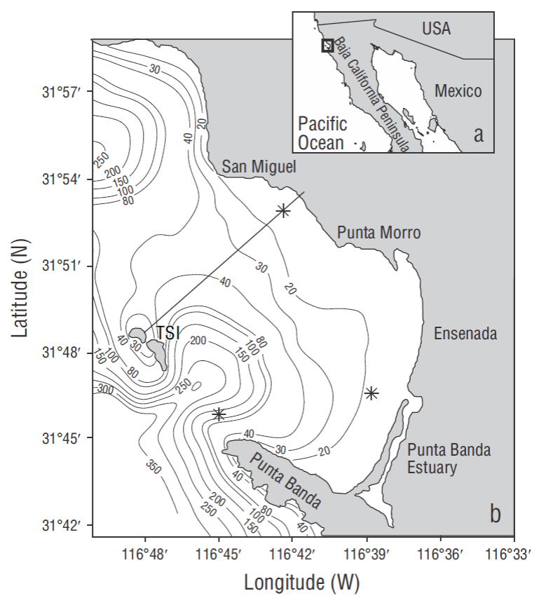
Figure 1 Study area: (a) Todos Santos Bay and (b) detailed view of the bay and bathymetry smoothed in ETOPO1. The asterisks represent the points on the grid where sea level time series were constructed. TSI stands for Todos Santos Island.
The California Current System
The California Current System (CCS) is formed by the equatorward California Current (CC), the seasonal surface coastal current (SCC), and northward subsurface countercurrent (SSC) (Lynn and Simpson 1987). The CC is the eastern part of the anticyclonic gyre in the North Pacific, which is characterized by its shallowness (0-300 m). This current transports cool, less saline waters with high dissolved oxygen levels from the polar regions to the equatorial zone. The average CC velocity is typically less than 25 cm s-1 (Reid and Schwartzlose 1962).
Geostrophic studies (Lynn and Simpson 1987, Strub and James 2000) showed that during spring and summer SCC flows towards the equator off California and the northern Baja California Peninsula (from 30ºN). During autumn and winter, SCC is inverted near the coast. By contrast, SSC flows northward at velocities between 4 and 8 cm s-1 at ~200 m depth during most of the year (Barton and Argote 1980). The formation of SCC is attributed to multiple local upwelling fronts (Strub and James 2000). Numeric studies showed that in order to develop velocity cores for SCC and SSC, the meridional variability of the Coriolis parameter f (β plane) and the alongshore component of wind stress need to be estimated. The β effect allows the offshore propagation of free waves (e.g., Rossby waves), modifying the density structure and contributing to the formation of an alongshore pressure gradient that contributes to the development of SSC along the eastern boundary (Batten 1997). Off the northern Baja California coast, between 31ºN and 32ºN, the SCC and SSC are unstable and cause great variability in the region (Mateos et al. 2013). Variability in water circulation off the northern Baja California coast has an impact on water circulation variability in TSB (Mateos et al. 2009).
Atmosphere
There are 2 relevant systems acting together that regulate wind seasonality along the California and Baja California coasts. The first is a high-pressure center located in the North Pacific, to the west of the coast of California, and it can shift between 28ºN/130ºW (in winter) and 38ºN/150ºW (in summer). This high-pressure center is persistent all year round, and it is more intense during summer but weakens during winter as it moves (Reid et al. 1958, Castro et al. 2006). The second is a low-pressure center markedly settled over the continent, northeastern Baja California, during summer; this is a semi -permanent system with a wider range in seasonal variability (Reid et al. 1958). Both systems are responsible for the northwesterly winds occurring during the warm months of the year.
Todos Santos Bay
There is a sea breeze circulation system in TSB, but this system is dominated by the circulation of synoptic winds blowing in a southeastern direction parallel to the coast of the Baja California Peninsula (Álvarez 1977, Parés 1981, Pavía and Reyes 1983). Two circulation systems were identified by a numeric study, forced with the CCS and stationary wind, for the summer circulation in TSB: the internal system, corresponding to the shallow section of the bay, and the external system, corresponding to the deep section of the bay. The external system consists of an intense, southward flowing current and it is limited by the 35- m isobath. The internal system has 2 circulation structures. The first structure consists of an anticyclonic circulation that covers the entire bay and produces a large eddy. This eddy grows and splits, originating the second structure, which consists of 2 eddies circulating in opposite directions and of which the original anticyclonic eddy is limited to the northern portion of the bay. This process occurs approximately every 3 to 5 days. The circulation variability was attributed to variations in transport at the mouths of the bay due to eddies occurring outside TSB (Mateos et al. 2009).
Filonov et al. (2014) identified a current amplification and attenuation pattern with a 3-day period from current observations during 2007, and it was consistent with the numeric study described by Mateos et al. (2009). However, Filonov et al. (2014) did not find the same circulation pattern found in the numeric study for the area near San Miguel; measurements revealed a predominant northwestern direction, whereas the model revealed a southeastern direction. The circulation oscillations observed from measurements and numeric studies have not been explained. The main objective of this study is to analyze the mechanisms that could explain this variability. To accomplish this, we analyzed the outputs of a tridimensional and baroclinic numeric model, with high horizontal and vertical resolution, forced with non-stationary wind, heat fluxes, and the CCS.
Materials and methods
The Regional Ocean Modeling System (ROMS) used for this experiment was developed by the University of California at Los Angeles, Rutgers University, and the Research Institute for French Development (IRD, French acronym). The ROMS 3.6 version used for this study is managed by Rutgers University; its code can be obtained at https://www.myroms.org/. ROMS is a tridimensional free-surface model that uses vertical S coordinates and horizontal curvilinear coordinates. It solves momentum equations with hydrostatic approximations and the temperature and salinity equations, and it uses a state equation that correlates pressure, temperature, and salinity with density.
The horizontal boundary conditions were imposed on the the temperature, salinity, and velocity fields. For computational efficiency reasons, ROMS solves momentum equations using a split time scheme (external and internal modes), which requires a special treatment and coupling between the barotropic (fast) and baroclinic (slow) modes. The free surface and vertically integrated momentum equations are calculated in a finite number of barotropic time steps within each baroclinic time step. In the two- and three-dimensional equations, a third-order finite-differences approximation is adopted for the predictor (Leap-Frog) and corrector (Adams-Molton), which is robust and stable (Shchepetkin and McWilliams 2005). On the horizontal coordinate, the model discretizes equations over a grid in curvilinear orthogonal coordinates, for implementations in Cartesian, polar, and spherical coordinates. On the vertical coordinate, equations are discretized over a changing topography using vertical coordinates that follow the topography (generalized “S” coordinates).
All model forcings and configurations were built based on climatologies, except wind stress, which was treated as described by Mateos et al. (2013). The daily wind stress and heat flux data were obtained from the North America Regional Reanalysis with a spatial resolution of 32 km.
The initial conditions and daily forcings in the open boundaries were obtained from a previous model validated by Mateos et al. (2013) . The formerly mentioned model was executed with 2 nested grids. The parent grid was compared with previous studies that analyzed observations with different techniques and spatiotemporal resolutions (Barton and Argote 1980, Gómez-Valdez 1983, Espinosa-Carreón et al. 2012). The child grid was compared with one-year measurements carried out by deep-water mooring. The initial and boundary conditions were taken from the child grid outputs.
This study has higher horizontal and vertical resolution than the experiment presented by Mateos et al. (2013). Thus, a grid was constructed with 170 × 340 cells on the horizontal coordinate, with an average resolution of 150 m, and 30 sigma levels were used on the vertical coordinate. In addition, a baroclinic time step set to 30 s was used to avoid violating the Courant condition due to increased resolution.
Results
Temperature and elevation of sea level fields for August were analyzed. The sea level elevation monthly average (Fig. 2) showed water accumulation in the region between Ensenada and the Punta Banda Estuary (E-PBE). Average water level decreased towards the northern mouth of the bay, with a 0.5-cm average difference between the mouth and the E-PBE region. In general, mean cyclonic circulation was observed covering the entire bay at 5 m depth (Fig. 2). This current pattern is consistent with the subtidal currents obtained from 2 high-frequency radars (Flores-Vidal et al. 2015). The mean subtidal current field showed that observed magnitudes were lower than 5 cm s-1, which is consistent with the model. Flores-Vidal et al. (2015) attribute the subinertial current behavior in the bay to the effects of the synoptic currents and/or to the synoptic wind field. Another important feature found in mean flow are 2 cyclonic eddies in TSB and a cyclonic circulation at the mouth close to TSI.
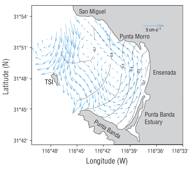
Figure 2 Average sea level elevation (isolines, centimeters) and current velocity at 5 m depth for August. An increased rise in sea level towards the south is shown.
Instant elevation fields showed that water accumulation in the southern region of the bay was released within approximately 3 to 5 days. For example, the evolution for sea level and instant velocity fields at 5 m depth were shown for 2 and 5 August (Fig. 3 a, c, respectively). In addition, to elucidate on the vertical structure, a vertical temperature section is shown for the area close to the northern mouth (Fig. 1), down to 20 m depth, during these 2 days (Fig. 3 b, d). On 2 August, the sea level structure (Fig. 3a) was very similar to the mean structure; elevation was highest in the section located in the E-PBE region and decreased towards the northern mouth of TSB. The velocity field showed a cyclonic eddy at the center of TSB and an anticyclonic one to the north. The latter, pre-vented the outward flow of water through San Miguel. On the vertical scale, the temperature structure was almost homogenous. The 6 ºC isotherm rose from 14 m near TSI up to the surface at the coast, forming a horizontal front with an approximate difference of 4 ºC in 7 km. As expected, due to the conditions, current velocities in TSB had a strong barotropic component (not shown).
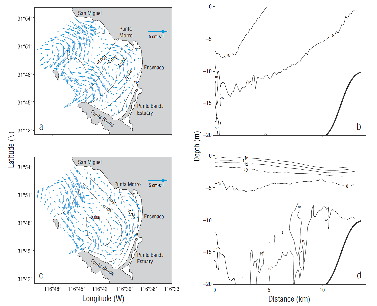
Figure 3 Sea level elevation and wind fields and instantaneous temperature sections at 2 different times. Sea level elevation (m) and the associated velocity field are shown for 2 August (a) and 5 August (c). The temperature (°C) vertical section is shown for 2 August (b) and 5 August (d), and the section goes from Todos Santos Island to the coast off San Miguel.
For 5 August maximum elevations were found along the west coast and decreased towards the western mouth of TSB (Fig. 3c) . On the other hand, sea level decreased by almost 0.3 cm in the E-PBE region, whereas in the San Miguel-Punta Morro region sea level increased by approximately 0.7 cm. The velocity field showed 2 anticyclonic eddies that covered almost all of TSB. The cyclonic eddy observed on day 2 at the northern mouth of TSB moved west-ward. Also, a small anticyclonic eddy (~2- km diameter) was observed to the south of Punta Morro. The layout of the previously mentioned eddies favored the outward flow from TSB through San Miguel. The vertical temperature section shows that the water column was well stratified in the upper 5 m. Isotherms at the surface decreased towards the coast (warm water close to the shore). Unlike day 2, day 5 had an important baroclinic component, which was also observed in the velocity field (not shown).
Additionally, the vertical transects for the western mouth were plotted for the same days (2 and 5) that were previously analyzed (not shown). The western mouth of TSB reached depths greater than 300 m. A similar stratification behavior as the one seen in the northern mouth was observed. However, for day 2, the homogenous layer was only 5 m deep.
For each one of the 3 grid points in the bay (Fig. 1, asterisks), sea level time series were constructed considering the same criteria. The first was located to the south of San Miguel, the second at the western mouth of TSB, and the third off Punta Banda Estuary (not shown). The linear tendency was removed from the time series, so values ranged around zero. In general, without removing the linear tendency, sea level was lower off San Miguel than off Punta Banda Estuary (not shown). The sea level time series showed that when sea level decreased off Punta Banda Estuary and at the western mouth, sea level increased off San Miguel (Fig. 4a). The Pearson correlation between the time series for Punta Banda Estuary and San Miguel was -0.76 (P = 1.14 × 10⁻⁶), whereas for the western mouth and San Miguel it was -0.54 (P = 0.001); thus, the null hypothesis, which states that the 2 series have no correlation, was rejected for both comparisons. For elevation of sea level, the Pearson correlation between the western mouth and Punta Banda Estuary was 0.26 (P = 0.15), so the null hypothesis (95% confidence interval) was not rejected.
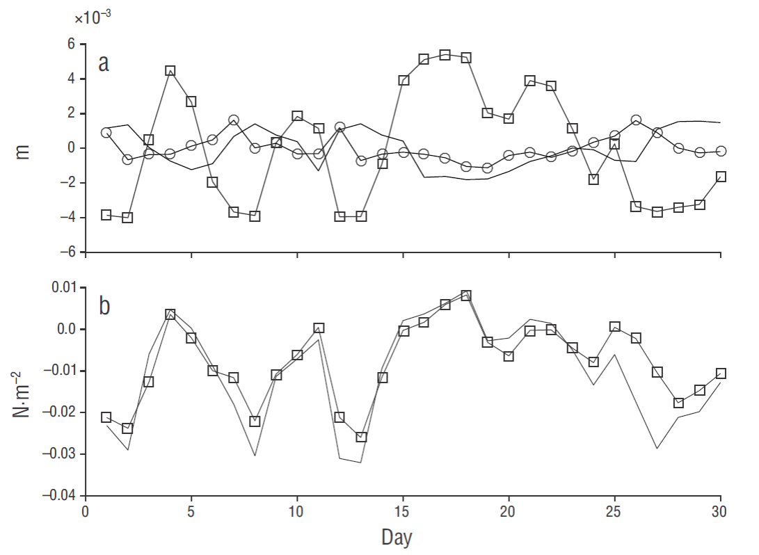
Figure 4 Time series of elevation of sea level (with no linear tendency) (a) and the wind stress component parallel to the coast (San Miguel-Punta Morro) (b) for the sites in Figure 1: the site close to San Miguel (empty squares), the western mouth of Todos Santo Bay (empty circles), and the site near Punta Banda Estuary (continuous line).
To determine the effect of wind, a time series for the wind-stress (used by the model) component parallel to the coast (San Miguel-Ensenada) was plotted for the same points considered in the sea level time series (Fig. 4b). The correlation between wind stress and sea level elevation was 0.95 (P = 1.9 × 10⁻¹⁵) and -0.83 (P = 1.3 × 10⁻⁸) for San Miguel and Punta Banda Estuary, respectively.
A complex empirical orthogonal function (CEOF) analysis was applied to the sea level elevation data corresponding to August. This analysis is a modification to the empirical orthogonal functions (EOF), and consists in adding a quadrature function as a complex number to the data. Thus, the real part is the original data and the Hilbert transform is the complex part.
The CEOF analysis for elevation of sea level showed that the first 2 modes explained close to 87% of the variance. The first CEOF mode (Fig. 5) explained 66.5% of the variance. In the spatial structure (Fig. 5a), relatively higher elevation was observed for the Punta Banda Estuary region, and the central and southern parts of the bay. A depression in sea level was observed off Ensenada and at the western mouth of TSB. The phase (Fig. 5b) showed propagation of elevation from the Punta Banda Estuary region to the northern mouth of the bay. The temporal structure of the mode (Fig. 5c) showed peaks of approximately 3 days, similar to what was found in measurements (data) by spectral analysis of sea level and currents (Filonov et al. 2014).
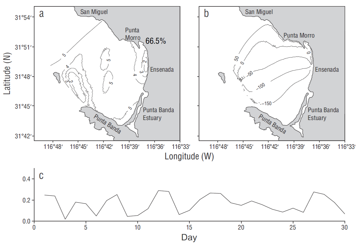
Figure 5 First mode of the complex empirical orthogonal function analysis of elevation of sea level for August, which explains 66.5% of the variance: (a) spatial structure of elevation amplitude normalized with variance, (b) spatial structure of the phase (each outline represents 50º), and (c) temporal structure of the mode.
The second CEOF mode (Fig. 6) explained 20.3% of the variance in the elevation field for August. In the spatial structure (Fig. 5a), differently to what was observed in the first mode, the highest relative elevations were found in the western mouth of the bay and off Ensenada. The lowest elevations were found in the area off Punta Banda Estuary and the central part of the bay. The propagation of elevation went from the western mouth of the bay towards the coast of Ensenada (Fig. 6b). On the other hand, the temporal structure for this mode (Fig. 6c) showed peaks of approximately 5 days. However, 2 or 3-day peaks were identified at the end of the month.
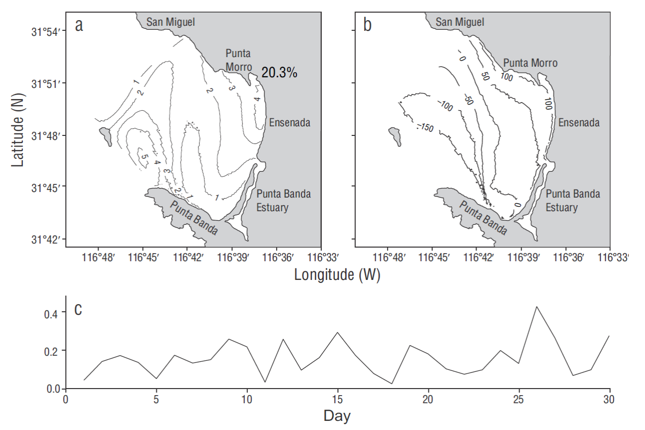
Figure 6 Second mode of the complex empirical orthogonal function analysis of elevation of sea level for August, which explains 20.3% of the variance: (a) spatial structure of elevation amplitude normalized with variance, (b) spatial structure the phase (each outline represents 50º), and (c) temporal structure of the mode.
Discussion
The results show evidence that wind, mainly southeasterly winds, caused water transport to the southeastern part of the bay. As a result, sea level in the E-PBE region increased, since Punta Banda Estuary forms a water flux barrier. More-over, off the San Miguel-Punta Morro coasts, upwelling of cold water occurred because of the southward water transport. This is consistent with what was reported in previous studies (Mateos et al. 2009). Due to upwelling of cold water in the San Miguel-Punta Morro region, coastal water flux is expected to move southeast (as seen in Mateos et al. 2009). In this study, water velocity in the San Miguel-Punta Morro region showed a northeastern direction, similar to what was found from measurement studies (Filonov et al. 2014). This suggests that the numerical experiment with stationary wind favors geostrophy, which considerably modifies the mean velocity field in the bay.
The results suggest that changes in sea level modify the temperature vertical structure and horizontal velocity fields. These changes in sea level occur in the same periodicity (3-5 days) as that for the reported variations in the velocity fields (Mateos et al. 2009, Filonov et al. 2014), suggesting that water accumulation release in the E-PBE region causes this variability.
The high correlation between elevation of sea-level and wind-stress (0.95 and -0.86) indicates that the intensification and weakening of the wind lead to the accumulation and release of water in E-PBE, respectively. However, in the previous numeric study, which was forced with stationary wind, water release was observed to occur with a similar periodicity. This is due to the fact that the numeric study was forced with CCS, as was done in the present study. Variability occurring in CCS is also associated with variability in wind stress (Strub and James 2000); that is, data on wind variability is included in CCS in both experiments.
The EOF analysis confirmed the propagation (release) to south of the free surface (elevation of sea level) towards the northwest of the bay, explaining 66.5% of the variability. On the other hand, the second mode (20.3%) suggests that free sea -surface variability in TSB is partly due to disturbances in the external part of the bay. This is consistent with the correlation found between elevations of the western mouth of TSB and San Miguel. Furthermore, the lack of correlation between the western mouth and Punta Banda suggests different mech-anisms that modify the temperature vertical structure off San Miguel. Disturbances in the external part of the bay can explain the variability reported in the study using stationary wind (Mateos et al. 2009).
This study correlates variability of velocity fields with sea level changes. The accumulation of water in the E- PBE region was caused by water transport from the northern part of the bay driven by wind-stress. Water accumulation is released every 3 to 5 days and propagates as a wave towards the northern part of the bay, modifying the velocity field and thermal structure at TSB. The periodicity of wave propagation is a result of the weakening of local winds and disturbances in the external part of TSB.

