Introduction

The main challenge for research on costal CO₂ flux (FCO₂) is to have enough data to identify the processes controlling its variability. The difference between partial pressure of carbon dioxide (pCO₂) in the ocean surface (pCO_2W) and pCO₂ in the atmosphere (pCO_2A) defines the direction of gas exchange. FCO₂ magnitude is a function of this difference and gas transfer velocity, which is parameterized as a function of wind speed. This speed is of great importance for the air-water gas exchange (^{Takahashi et al. 2002}). Physical and biological forcings such as mixing by wind, waves, phenomena associated with tides, advection, vertical displacement of the thermocline, photosynthesis, respiration, and air-water exchange drive substantial variations in pCO_2W over time, from periods of hours to interannual periods (^{DeGrandpe et al. 1998}). In addition, pCO_2W changes with mesoscale (^{Turi et al. 2014}) and sub-mesoscale (^{Klein and Lapeyre 2009}) processes, such as eddies and meanders in combination with physiographic (e.g., points, capes, islands) and bathymetric heterogeneity (^{Laruelle et al. 2014}). This leads to a complex mosaic of pCO_2W changes in space and time, and substantial measurement efforts are thus needed to reliably determine the role of the region as a CO₂ source or sink (^{Turi et al. 2014}).

Coastal waters in the California Current System have been characterized, using different methodologies, to define their role as carbon sources or sinks (^{DeGrandpe et al. 1998}; ^{Friederich et al. 2002}; ^{Chavez et al. 2007}; ^{De La Cruz-Orozco et al. 2010}; ^{Pennington et al. 2010}; ^{Evans et al. 2011}, ²⁰¹⁵; ^{Hales et al. 2012}; ^{Fiechter et al. 2014}; ^{Turi et al. 2014}; ^{Muñoz-Anderson et al. 2015}; ^{Mariano-Matías et al. 2016}). However, there are uncertainties in the direction of FCO₂ in this system. ^{Takahashi et al. (2009)} reported that the climatological mean annual value for the oceanic area off southern California and northern Baja California is close to equilibrium.

^{Hales et al. (2012)} predicted coastal pCO _2W from remote-sensing data for the Pacific region between 22ºN and 50ºN (from near the entrance to the Gulf of California to southern British Columbia, 30 to 370 km offshore) and characterized this area as a sink of atmospheric CO₂ with an annual average value of 1.8 mmol C m^-2 d^-1. ^{Chavez et al. (2007)}, however, reported that the same area is a source of about 0.07 mmol C m^-2 d^-1 (which is practically zero). De La ^{Cruz-Orozco et al. (2010)} used in situ sea-surface data to report that the area off the Baja California Peninsula (~30 to ~300 km from the coast) acted as a source of CO₂ from October 2004 to October 2005, with an average of 1.12 mmol C m^-2 d^-1. On the other hand, ^{Mariano- Matías et al. (2016)} reported that, according to the average for the years 2004-2011, the area off Baja California (>28ºN) was a sink of atmospheric CO₂. The complex dynamics in this area, which vary rapidly over short distances and at high frequencies and are affected by different events at different scales, may be the cause of these uncertainties (^{Chavez et al. 2007}).

Phenomena such as coastal upwelling, El Niño/Southern Oscillation (ENSO), and most recently “The Blob” (strongly positive temperature anomalies in the NE Pacific) affect the coastal zone in the California Current System (^{Wooster 1960}, ^{Mantua et al. 1997}, ^{Bond et al. 2015}). Wind-generated upwelling events show seasonal variability and bring cold, nutrient-rich waters along the coast, from Washington to Baja California (^{Huyer 1983}). These upwelled waters have high pCO_2W values, which are generally limited to a coastal band (^{Pennington et al. 2010}). ^{Lara- Lara et al. (1980)} and ^{Álvarez-Borrego and Álvarez-Borrego (1982)} reported that upwelling events off northern Baja California are characterized by an intensification-relaxation sequence with periods of about 2 weeks. This upwelling sequence may cause pCO_2W variations, with greater values during intensification than during relaxation events.

^{Lynn and Simpson (1987)} observed that in early autumn, wind speed declines and coastal upwelling weakens. In late autumn and early winter, there is a surface coastal countercurrent that inhibits upwelling (^{Hickey 1998}). ^{Mirabal-Gómez et al. (in press)} reported that the satellite derived chlorophyll climatology for the region off San Diego, California, and off San Quintín, Baja California (~200 km to the south of our buoy location), showed different biological conditions for 2 seasons: strong upwelling season and weak upwelling season. For the region off San Diego, the strong upwelling season occurred from March to June and the weak upwelling season during the rest of the year. The strong upwelling season for the region off San Quintín occurred from February to June. It is likely that pCO_2W is higher during the strong upwelling season than during the weak upwelling season.

During El Niño events sea surface temperature (SST) increases and phytoplankton biomass and production decrease (^{Reid 1962}, ¹⁹⁸⁸; ^{Putt and Prézelin 1985}; ^{Torres-Moye and Álvarez-Borrego 1987}; ^{Fargion 1989}; ^{Thomas and Strub 1990}; ^{Lynn et al. 1998}; ^{Kahru and Mitchell 2000}, ²⁰⁰²) . Because stratification is stronger, pCO_2W may be lower during an El Niño event than during “normal” conditions. Events with anomalously low SSTs (La Niña) may have the opposite effect, with relatively high pCO_2W.

Offshore SST in the NE Pacific was remarkably warm during the 2013-2014 winter season (^{Bond et al. 2015}); NA Bond dubbed this warm phenomenon the Blob. This marine heat wave persisted through 2013-2015 due to atmospheric teleconnections spanning the entire North Pacific (^{Di Lorenzo and Mantua 2016}), and its influence on the southern California Current System coastal waters ended by late November 2015 (http://www.ospo.noaa.gov). The Blob depressed the thermocline and caused high stratification from the summer in 2014 to the 2015-2016 winter season (^{Zaba and Rudnick 2016}), and it likely caused relatively low pCO_2W values.

Oceanographic cruises provide a limited number of observations to describe time variations. Data obtained from instruments mounted on moored buoys (e.g., pCO_2W measurements) are important additions to data obtained from cruises, and play a key role in getting a better understanding of time variability with spectra ranging from high-frequency periods (e.g., diurnal) to interannual periods. Related measurements, such as measurements of pCO_2A, SST, salinity, and wind, may allow us to analyze the drivers of pCO_2W variability (^{Friederich et al. 1995}, ^{Hofmann et al. 2011}, ^{Sutton et al. 2014}). Time series with high-resolution data are particularly needed to explore the questions about short-term variability at fixed locations that help discern the processes taking place in the area (^{Bates et al. 2014}, ^{Sutton et al. 2014}).

Moored Autonomous pCO₂ (MAPCO ₂) systems have been deployed off the central and southern California coasts (^{Friederich et al. 1995}, ^{Sutton et al. 2014}). Only one such system was deployed in the California Current System region off northern Baja California, and it provided data for only one year (^{Muñoz-Anderson et al. 2015}). The California Current exhibits particular dynamics in this area. ^{Peláez and McGowan (1986)} used Coastal Zone Color Scanner chlorophyll data to describe the Ensenada Front located at the southern limit of the Southern California Bight (Fig. 1). This front extends about 500 km offshore. Water north of the front is eutrophic, cold, and less saline, but to the south, it abruptly becomes oligotrophic. An onshore flow characterizes the front and, at the coast, it divides into a branch to the north and another one to the south (Fig. 1). The front reaches its south-ernmost position (off our bouy location) by mid- or late summer (^{Peláez and McGowan 1986}). ^{Santamaría-del-Ángel et al. (2002)} reported that the latitudinal position of the front presents interannual variations, and during an El Niño event it moves northward to 34ºN. This latitudinal variation of the front may not have a particular discernible effect on pCO_2W when an El Niño event occurs other than that of El Niño itself.

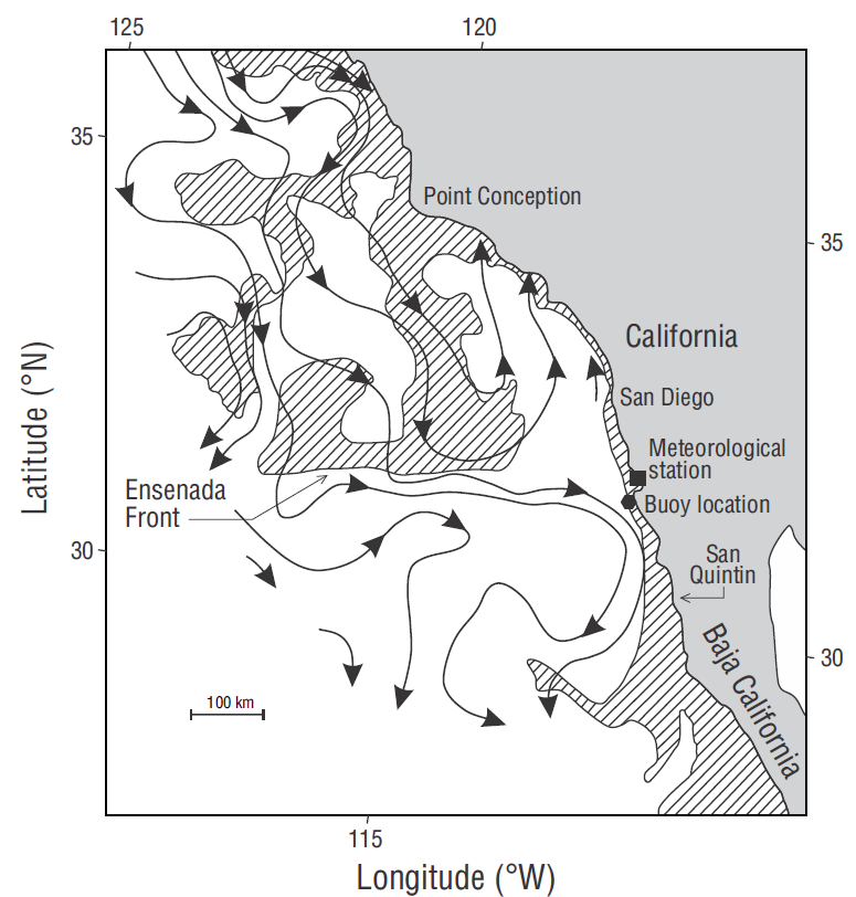
Figure 1 Location of the moored buoy 5 km off Punta Banda, Baja California (Mexico). The geostrophic flow (arrows) shows the Ensenada Front. Shaded areas represent relatively high chlorophyll concentrations and clear areas represent oligotrophic conditions (chlorophyll data are from the Coastal Zone Color Scanner) (figure taken from ^{Álvarez-Borrego 2004}, who adapted the figure from ^{Peláez and McGowan 1986}). 

There has been little research on pCO_2W dynamics in the Ensenada Front region. This region features strong upwelling events with low SST (<14 ºC), relatively low salinity (<34.0), and high pCO_2W values (~700 atm), resulting in an export of excess CO₂ to the atmosphere. By contrast, ^{Muñoz-Anderson et al. (2015)} reported that during the weak upwelling season, it is characterized by intermediate surface temperatures and low pCO_2W values (down to ~300 µatm), resulting in a CO₂ sink. These authors used a MAPCO₂ system to analyze the seasonal changes of pCO_2W and FCO₂ in one year (2009), without any reference to high frequencies (i.e., diurnal changes) or interannual changes. They reported average daily fluxes of 0.6 ± 0.1 mmol C m^-2 d-1 for winter, 2.8 ± 0.3 mmol C m^-2 d-1 for spring, 0.3 ± 0.1 mmol C m^-2 d-1 for summer, and -0.3 ± 0.03 mmol C m^-2 d-1 for autumn; the positive values indicate fluxes from water to air and vice versa. ^{Muñoz-Anderson et al. (2015)} concluded that, according to the annual average, the buoy location off Ensenada was a source of CO₂ to the atmosphere. However, it is desirable to extend the time series to include interannual changes and thus have a better description of the effects of the various factors affecting pCO_2W variability. High-frequency variations may also be of interest. In this work, time series spanning several years are analyzed (August 2008 to August 2015) for a coastal location in the Ensenada Front region. Some of the physical phenomena that occurred during this period were diurnal breezes, seasonal upwelling, El Niño 2009-2010, La Niña 2010-2012, the Blob 2014-2015, and the El Niño 2015. The aim of this study was to describe SST, pCO _2W, and FCO₂ variations, from semidiurnal to the interannual scales, and to identify their drivers.

Materials and methods

Calculation of FCO₂

Flux (FCO₂) was calculated according to ^{Liss and Merli-vat (1986)}: FCO₂ = k × K´ × ( ΔpCO₂) (mmol m^-2 h^-1; here, units are per hour because of our pCO_2W data resolution). The k parameter is the gas transfer velocity as a function of (U₁₀) and it is expressed as k = 0.251(Sc/660)^0.5 × (U₁₀)² (^{Wanninkhof 2014}), where Sc is the Schmidt number as a function of temperature; K´ is CO₂ solubility as a function of temperature and salinity (for details, see Table 2 in ^{Wanninkhof [2014]}); and ΔpCO₂ is pCO_2W minus pCO_2A. We integrated FCO₂ to obtain values in per day and build Figure 2c.

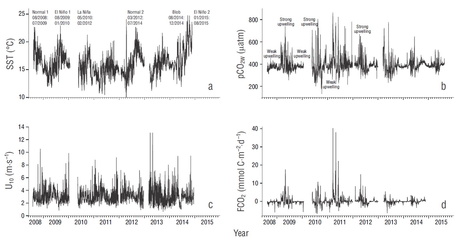
Figure 2 Time series of (a) sea surface temperature (SST), (b) CO₂ partial pressure at the ocean surface (pCO_2W), (c) wind speed at 10 m above sea level (U₁₀), and (d) air-water CO₂ flux (FCO₂). Data for SST and FCO₂ are from August 2008 to November 2014, and for pCO_2W from August 2008 to August 2015. Legends in the upper panel indicate periods and their duration (month/year to month/year). Data for SST, pCO_2W, and U₁₀ are given for every 3 h, and for FCO₂ data are given as per day. 

Results

There was a large spectrum of SST, pCO_2W, U ₁₀, and FCO₂ variations, with periods as short as few hours and as large as interannual time frames (Figs. 2-5). Unfortunately, the sensors did not work for relatively long periods in 2008, 2010, 2013, and 2015. Nonetheless, there were enough data to run spectral analysis and to test for differences between conditions: daylight vs night, strong upwelling vs weak upwelling seasons, El Niño vs La Niña, and Blob vs no Blob.

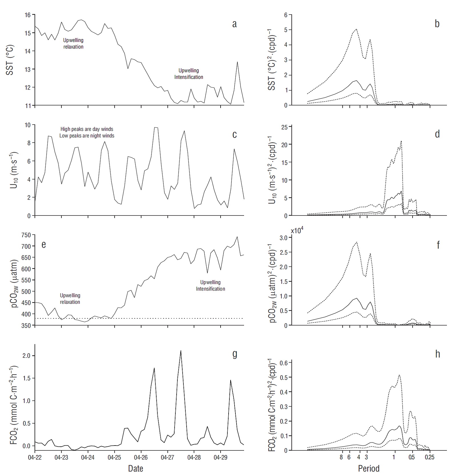
Figure 3 Eight day-time series of (a) sea surface temperature (SST), (c) wind speed at 10 m above sea level (U₁₀), (e) CO₂ partial pressure at the ocean surface (pCO_2W), and (g) air-water CO₂ flux (FCO₂). Dates on the horizontal axes are for April 2011, and ticks indicate the beginning of the day (midnight). High peaks in (c) correspond to diurnal winds and low peaks to nocturnal winds. The horizontal dotted line in (e) indicates CO₂ partial pressure in the atmosphere (pCO_2A) for 2011 (391 µatm). Power spectra are shown on the right panels: horizontal axes indicate the corresponding periods in days, and broken lines indicate 95% confidence intervals. 

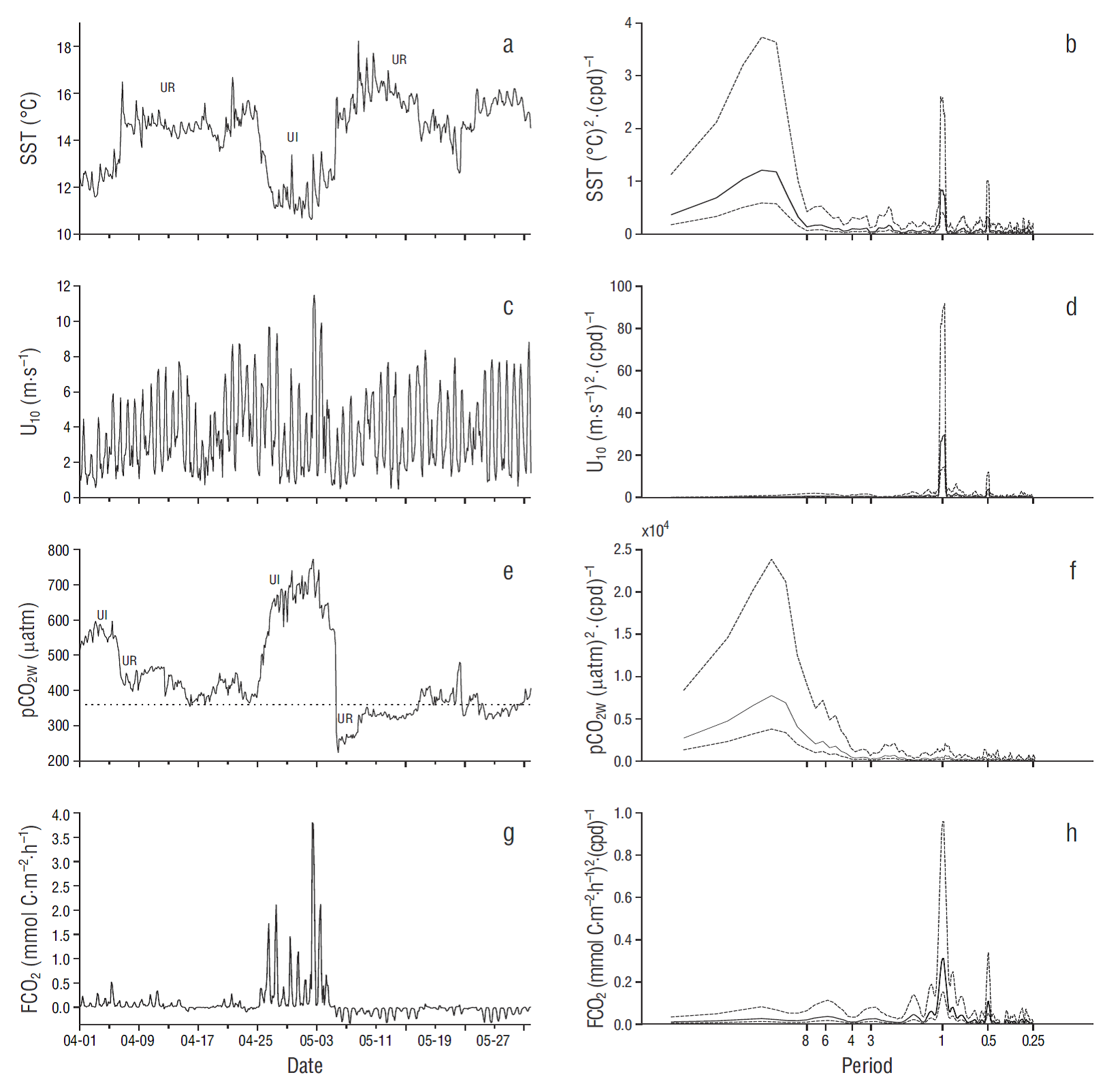
Figure 4 Two-month time series of (a) sea surface temperature (SST), (c) wind speed at 10 m above sea level (U₁₀), (e) CO₂ partial pressure at the ocean surface (pCO_2W), and (g) air-water CO₂ flux (FCO₂). Dates on the horizontal axes are for April and May 2011, and ticks indicate the beginning of the day (midnight). The horizontal dotted line in (e) indicates CO₂ partial pressure in the atmosphere for 2011 (391 µatm). UI means upwelling intensification and UR means upwelling relaxation. Power spectra are shown on the right panels: horizontal axes show the corresponding periods in days and broken lines indicate 95% confidence intervals. 

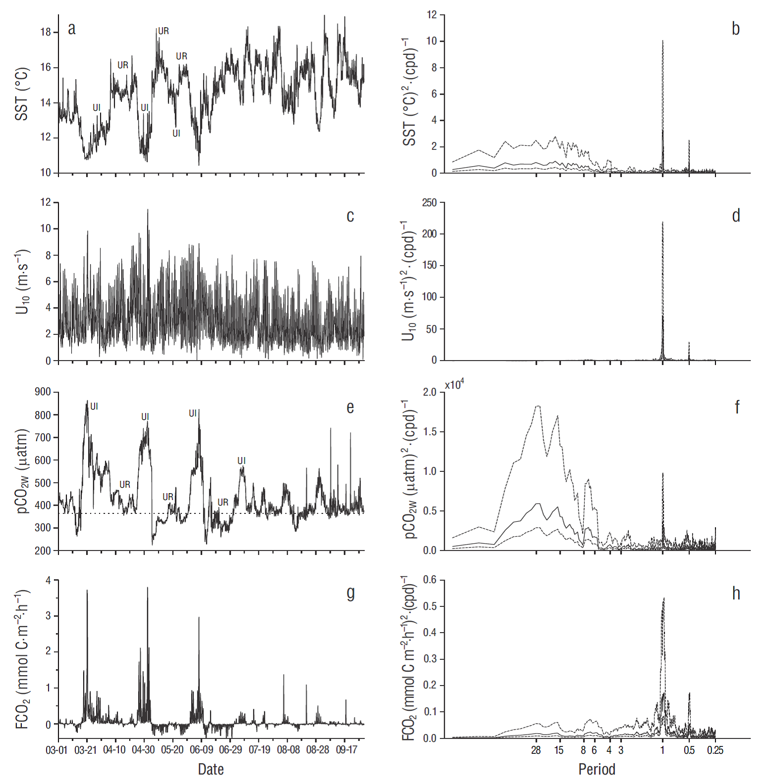
Figure 5 Seven-month time series of (a) sea surface temperature (SST), (c) wind speed at 10 m above sea level (U₁₀), (e) CO₂ partial pressure at the ocean surface (pCO_2W), and (g) air-water CO₂ flux (FCO₂). Dates on the horizontal axes are for March-September 2011, and ticks indicate the beginning of the day (midnight). The strong upwelling season is from March to June. The horizontal dotted line in (e) indicates CO₂ partial pressure in the atmosphere for 2011 (391 µatm). In (a) and (e), UI means upwelling intensification and UR means upwelling relaxation. Power spectra are on the right panels: horizontal axes show the corresponding periods in days, and broken lines indicate 95% confidence intervals. 

In general, at our sampling location, pCO_2W showed a tendency towards oversaturation in March-August (the strong upwelling season) and was near equilibrium or under saturation levels in September-February (the weak upwelling season) (Fig. 2b). Unfortunately, it was not possible to see the effect of El Niño conditions on air-sea gas exchange for the first half of 2010. Nevertheless, in August-December 2009 (with El Niño 1, and during a weak upwelling season) pCO_2W and FCO₂ values were relatively low, with a tendency to reach equilibrium (Fig. 2b, d). The pCO_2W range for August-December 2009 was from 313 µatm (September) to 551 µatm (August), the latter being a very high value with respect to what is expected for El Niño conditions. These values corresponded with the SST values of 17.9 and 12.9 ºC (a very low value for these conditions), respectively, and with the FCO₂ values of -1.9 mmol C m^-2 d^-1 and 1.4 mmol C m^-2 d^-1, respectively.

The largest pCO_2W and FCO₂ variations occurred in 2011, under La Niña conditions (Fig. 2b, d). During this period, pCO_2W and FCO₂ maximum values were higher, and minimum values were lower, than during “normal,” El Niño, and the Blob conditions. The pCO_2W range for our whole data set was from 131 µatm (October 2010) to 864 µatm (March 2011). These values corresponded to SST values of17.0 and 10.9 ºC, respectively, and with the FCO₂ values of -6.9 mmol C m^-2 d^-1 and 40.4 mmol C m^-2 d^-1, respectively (Fig. 2a, b, d).

During 2012, 2013, and the first half of 2014, under “normal 2” conditions, the lowest pCO_2W value was 232 μatm (May 2013) and the largest was 779 μatm (June 2013). The largest FCO₂ value during these years was 14.9 mmol C m^-2 d^-1 (April 2012) and the lowest was -6.5 mmol C m^-2 d^-1 (May 2013) (Fig. 2b, d). The largest pCO_2W value did not correspond with the largest FCO₂ value, mainly because of differences in wind intensity (Fig. 2b-d).

Starting in June 2014, the effect of the Blob on SST was clearly marked (see also http://www.ospo.noaa.gov). Sea surface temperature increased up to a maximum of 26.0 ºC in October 2014, whereas maximum values during October-November of other years were ~20.0 ºC (Fig. 2a). During the second half of 2014, the pCO_2W range was from 323 to 483 μatm, and the FCO₂ range was from near equilibrium to ~2.5 mmol C m^-2 d^-1, lower than the maximum FCO₂ value during “normal 2” conditions (Fig. 2b, d). During 2015, with El Niño 2 (EN2) event, the pCO_2W range was smaller than that in 2014. We did not have any SST data for 2015, so we were unable to calculate FCO₂ for that year.

In order to explore variability at different scales in more detail, time series were analyzed by segments of 8 d (diurnal variations and one upwelling intensification-relaxation sequence), 2 months (upwelling intensification-relaxation sequences), and several months (strong upwelling-weak upwelling seasons). Different periods were analyzed but those during La Niña conditions (2011) showed the highest variations. For this reason, examples were illustrated with data from 2011: 22-29 April (Fig. 3), 01 April-31 May (Fig. 4), and 01 March-30 September (Fig. 5). Power spectra for SST and pCO_2W tended to be similar at all scales, while those of wind speed and FCO₂ tended to be similar but different from those of SST and pCO_2W (Figs. 3-5).

In the case of the 8-d time series, SST was low and pCO_2W was high when there was an upwelling intensification event, and vice versa (Fig. 3a, e). During the first 3 d of this series, SST was relatively high (15.0-15.5 ºC), pCO_2W was relatively low (~400 µatm), and FCO₂ was close to equilibrium (Fig. 3a, e, g). From the fourth day on, SST decreased to ~11.0 °C, pCO_2W increased to ~µ700 μatm, and FCO₂ showed large diurnal variation (0.0 to ~2.0 mmol C m^-2 h^-1) because of wind variation. Lowest daily wind speed and FCO₂ values occurred at midnight and the highest in the afternoon (Fig. 3g). FCO₂ values were very low with weak winds in spite of high pCO_2W values (e.g., µ650 μatm) (Fig. 3c, e, g). The largest spectral density for wind speed (U₁₀) and FCO₂ was centered at a frequency of ~1 cycle per day, while for SST and pCO_2W it was centered at ~0.25 cycles per day (~4-d period) (Fig. 3). Both U ₁₀ and FCO₂ had a second spectral density peak centered at ~2 cycles per day (~0.5-d period) (Fig. 3c, d, g, h). Neither SST nor pCO_2W showed a significant component of variation at frequencies higher than ~0.67 cycles per day (~1.5-d period).

During the first ~25 d of the April-May time series (Fig. 4), ΔpCO₂ was mostly positive (not illustrated), and FCO₂ showed small positive values close to equilibrium (<0.5 mmol C m^-2 h^-1) in spite of the relatively high pCO_2W values (range: 400-600 µatm) (Fig. 4 e, g). The FCO₂ values during this first period were close to equilibrium because pCO _2W was high when wind speed was under 6 m s^-1, and they were close to pCO_2A when winds were relatively strong (>8 m s^-1) (Fig. 4c, e, g). In other words, during these first 25 d there was no correlation between wind speed and pCO_2W. In the following ~10 d, upwelling was intense (SST was <11 ºC), and pCO_2W values (400-800 µatm) were in general higher than during the previous days. This resulted in some large positive FCO₂ values (range: 0.01 to ~3.8 mmol C m^-2 h^-1), and large FCO₂ high-frequency variation in relation to wind variation (from <1 m s^-1 to >11 m s^-1) (Fig. 4c, e, g). During the last 26 d of this April-May time series, ΔpCO₂ was mostly negative (not illustrated), and FCO₂ showed small negative values close to equilibrium (from ~0.0 to -0.3 mmol C m^-2 h^-1). At the beginning of this last 26-d segment, pCO₂ reached high negative values, down to -170 µatm, but FCO₂ was close to equilibrium, again, because of weak winds (up to 5 m s^-1) (Fig. 6c, g). During these 2 months SST, U ₁₀, and FCO₂ had significant components of variation at ~1- and ~0.5-d periods. For U₁₀ and FCO ₂, diurnal and semidiurnal components of variation were the largest, with significant but much smaller low-frequency variations (corresponding to ~3, ~6, and ~15-d periods for FCO₂). The pCO_2W time series had very small components of variation at ~1- and ~0.5 -d periods. The largest spectral density for SST and pCO_2W was at ~0.07 cycles per day (~15-d period, possibly related to the upwelling intensification-relaxation sequence).

The 7-month time series showed that during March-June SST minima were <11 ºC, indicative of very strong upwelling events (Fig. 5a) . In August and September SST maximum values increased by ~2 ºC with respect to the maximum values from previous months, yet minima were still under 13 ºC (Fig. 5a), which indicates upwelling events during late summer, although less intense. The pCO_2W ranges were larger in spring (from the lowest minima of ~220 μatm up to the highest maxima of ~870 μatm) than in summer (from the lowest minima of ~300 μatm up to the highest maxima of ~590 μatm) (Fig. 5 e), indicating the strongest upwelling events occurred during spring. The FCO₂ values, both positive and negative, were larger in spring (from -0.5 to 3.8 mmol C m^-2 h^-1) than in summer (from -0.1 to 1.4 mmol C m^-2 h^-1) (Fig. 5 g) because of the more extreme pCO_2W values during spring, but also the larger U ₁₀ values (Fig. 5c, e). Furthermore, the FCO₂ large positive values persisted much longer in spring than in summer (Fig. 5g). At the 7-month scale all 4 variables (SST, U₁₀, pCO_2W, and FCO₂) had significant components of variation at ~1- and ~0.5-d periods (Fig. 5b, d, f, h) . The largest component of variation was the diurnal one for SST, U₁₀, and FCO₂ (Fig. 5b, d, h ,) though pCO _2W showed the largest variation at the 17- and 28-d periods (Fig. 5f).

There were significant differences in pCO_2W and FCO₂ when comparing periods under different conditions (i.e., day vs night, upwelling intensification vs upwelling relaxation, strong vs weak upwelling seasons, El Niño vs La Niña, and the Blob vs no Blob). In all types of comparisons, the Bayesian t test for pCO_2W and FCO₂ showed high probability that the medians of the groups were credibly different from each other.

When taking our whole data set, the FCO₂ integral and the corresponding standard error for each period (Fig. 2d) were as follows: “normal 1”, -4.7 ± 0.02 mmol C m^-2; El Niño 1, -57.0 ± 0.01 mmol C m^-2; La Niña, 257.0 ± 0.03 mmol C m^-2; “normal 2”, 2.2 ± 0.02 mmol C m^-2; and the Blob, 18.4 ± 0.01 mmol C m^-2. For the “normal 1” period, we had data for only 11 months and the pCO_2W range was smaller (~300 to 400 μatm) than for the “normal 2” period (~300 to 550 μatm), with the “normal 2” period presenting few ~700 μatm values during intense upwelling (Fig. 2b); this may explain the large difference between these 2 periods.

The FCO₂ averages for the day and night periods during strong upwelling seasons were 0.09 ± 0.09 mmol C m^-2 h^-1 and 0.03 ± 0.006 mmol C m^-2 h^-1, respectively. During the weak upwelling seasons FCO₂ averages were -0.03 ± 0.00 mmol C m^-2 h^-1 for the day, and -0.02 ± 0.00 mmol C m^-2 h^-1 for the night. In both cases there were significant differences between day and night.

Discussion

Ocean CO₂ outgassing is fast; it occurs during the first hours after the upwelled water reaches the surface (^{Turi et al. 2014}). At first, rising waters are supersaturated with respect to atmospheric CO₂ (high pCO_2W) but may quickly become undersaturated if a phytoplankton bloom occurs (^{Simpson and Zirino 1980}). At our MAPCO₂ location, during these first hours, the effects of outgassing and phytoplankton carbon uptake contributed to the reduction of pCO_2W. When upwell-ing relaxed, pCO_2W was low; it is possible that photosynthesis was high, continued that way for 4 to 5 days (see ^{Lara-Lara et al. 1980}), and decreased pCO_2W even more, causing negative FCO₂ values. During relaxation, gas exchange (negative FCO₂) and photosynthesis have opposite effects on pCO_2W, yielding relatively small negative pCO₂ values. This explains the larger maximum FCO₂ values compared to the absolute values of the negative ones (Fig. 2d). During the most intense outgassing (May 2011, Fig. 2d), FCO₂ was ~40 mmol C m^-2 d^-1, whereas phytoplankton integrated production was >1 g m^-2 d^-1 (^{Sosa-Ávalos et al. 2010}), equivalent to >80 mmol C m^-2 d^-1; this indicates that photo-synthesis is a stronger process than outgassing in the reduction of pCO_2W.

There was a strong dependence of FCO₂ on U ₁₀, through the gas transfer velocity (k), as expressed by ^{Liss and Merlivat (1986)} and ^{Takahashi et al. (2002)}. ^{Reyes and Parés (1983)} reported that wind data from our study area show the highest energies at diurnal and semidiurnal frequencies, giving evidence of the sea-land breeze and free-convection processes. When estimating FCO₂, pCO₂ is to the first power, and when estimating k, U₁₀ is to the second power; thus, wind speed has a larger impact than pCO₂ on the estimates of FCO₂ (^{Wanninkhof 2014}).

The upwelling intensification-relaxation sequence off northern Baja California, with periods of about 2 weeks (^{Lara-Lara et al. 1980}, ^{Álvarez-Borrego and Álvarez-Borrego 1982}), explains why the SST and pCO_2W spectral analyses showed components of variation with periods of ~15 d (Fig. 5b, f). However, SST had a very broad spectral band, probably because upwelling intensification and relax-ation events are not always equal in magnitude. ^{Álvarez-Borrego and Álvarez- Borrego (1982)}, using SST data, reported the occurrence of 10 intense upwelling intensification-relaxation events during 1979 at a site located 200 km south of our sampling point, with the most intense events occurring in July, when minimum surface temperatures were <11.0 ºC. Timing of the relative intensity of upwelling events therefore depends on the physiography and ocean dynamics of each particular coastal location.

Under warm conditions, the effect of upwelling is relatively weak, surface nutrients and dissolved inorganic carbon reach relatively low values, and phytoplankton abundance is low (^{Torres-Moye and Álvarez-Borrego 1987}, ^{Borges et al. 2005}, ^{Müller-Karger et al. 2005}), and this explains our relatively small pCO_2W and FCO₂ ranges during El Niño. The 2009-2010 El Niño event was of the central Pacific type (or El Niño Modoki) (^{Ashok et al. 2007}, ^{Lee and McPhaden 2010}). ^{Mirabal-Gómez et al. (in press)} reported that phyto-plankton biomass off San Diego, California, was lower during El Niño 2009-2010 than in 2011. According to ^{Fiechter et al. (2014)}, pCO_2W values are lower during El Niño Modoki than during “normal” conditions.

During El Niño Modoki and the Blob events, SST was high and CO₂ solubility was low. In the case of El Niño, this was due to the presence of warmer, high-salinity water from the equatorial Pacific (^{Schneider et al. 2005}). The Blob was a phenomenon with local heating of surface waters in the northeastern Pacific (^{Bond et al. 2015}). During El Niño, upwelling and some carbon uptake took place, but SSTs were higher and photosynthesis was lower than during “normal” conditions. Our FCO₂ data for the Blob in 2014 only covered the weak upwelling season, and local warming and reduced CO₂ solubility resulted in CO₂ outgassing. The El Niño 2015 was of the eastern Pacific type and its effect on our study area started in April of that year (http://www.ospo.noaa.gov). This El Niño added its effect to that of the Blob causing lower pCO_2W maxima than in 2014 (Fig. 2b).

The largest pCO_2W and FCO₂ variations (i.e., 131-864 μatm) in our time series occurred under La Niña conditions. During this period, pCO_2W and FCO₂ maxima were higher, and minima were lower, than during all the other periods. ^{Evans et al. (2011}, ²⁰¹⁵⁾ reported fluctuating pCO_2W values between 1,200 and <200 μatm for the Oregon coastal upwelling region under La Niña conditions. Compared to what happens under “normal” and warm conditions, during La Niña, the upwelling effect is stronger because water comes from deeper layers and is more enriched with dissolved inorganic carbon and nutrients, and this enhances CO₂ outgassing (^{Ishii et al. 2009}, ^{Heinze et al. 2015}) and increases photosynthetic carbon uptake (^{Barber and Chavez 1983}). Our highest pCO_2W values under La Niña conditions were about twice the equilibrium value, whereas most of the lowest values were around half that of equilibrium. Positive pCO₂ values were greater than absolute negative values, yielding larger positive than negative FCO₂ values.

Carbon uptake by photosynthesis is greater during relaxation than during intensification of upwelling events because phytoplankton uses nutrients more effectively during relaxation conditions (^{Barber and Ryther 1969}, ^{Lara- Lara et al. 1980}, ^{Wilkerson et al. 2006}, ^{Evans et al. 2015}). Therefore, when upwelling was intense, both pCO_2W and FCO₂ were high and carbon uptake was possibly low. When upwelling relaxed, pCO_2W was low and FCO₂ was negative, while carbon uptake was possibly high (e.g., several events in March-June, 2011) (Figs. 3-5).

It is important to consider the location of our buoy for concluding on the role of the area as a source or sink of carbon. Strictly speaking, the results of this work are only representative of this location. Extrapolating these results to a larger area is less reliable because variations through time depend on the location of the moored buoy. ^{Pennington et al. (2010)} illustrated the variation of pCO_2W and FCO ₂ off Monterey Bay, from coastal to offshore waters; they observed that FCO₂ was negative (air to water) near the coast and further offshore, but it was strongly positive (~1.0 mol C m^-2 yr-1) at ~20 km from the coast. The mean FCO₂ value at our sampling site (5 km from the coast) for the sampled period (2008-2014) was 0.04 ± 0.02 mol C m^-2 yr-1, with a large positive integrated value for La Niña period and a relatively large negative value for El Niño 1. Nonetheless, our FCO₂ average value is very small and close to equilibrium compared to the FCO₂ values for the large oceanic CO₂ sinks and sources (~10 mol C m^-2 yr-1; North Atlantic and Equatorial Pacific, respectively), as shown by ^{Takahashi et al. (2009)}. ^{Hernández-Ayón et al. (2010)} used “ships of opportunity” to study the CO₂ air-sea exchange off Baja California in the period 1993-2001 and concluded that, on average, this area is in equilibrium, which is in agreement with our results.

We estimated the pH ranges that correspond to our pCO _2W ranges. As ^{Park (1969)} indicated, knowing any 2 variables of the CO₂ system (pH, total alkalinity, dissolved inorganic carbon, pCO_2W), it is possible to calculate the whole dissolved inorganic carbon system (including HCO₃-, CO₃2-, percent saturation of calcite, etc.). Thus, we used ^{Lee et al.’s (2006)} global relationships (the expression for their oceanic region 1) to calculate total alkalinity values as a function of salinity, and with this property and pCO_2W we estimated the corresponding pH values. As mentioned above, the extreme pCO_2W values were 131 and 864 μatm and the corresponding pH values are 8.56 and 7.86 in the NBS scale; the equilibrium pH value for a pCO_2A of 400 μatm is 8.18. These pH values are 8.38, 7.68, and 7.99, respectively, in the seawater scale. The extreme pH values resulted from processes that occurred from below the surface (upwelling and photosynthesis) and only lasted for short periods of time (Fig. 2b). Organisms that dwell in these coastal waters have adapted during millennia to these kind of wide pH ranges. However, as anthropogenic input of CO₂ to the atmosphere continues, the pH equilibrium value around which these extreme values fluctuate will decrease, and this could have an impact on the biota.

In summary, processes such as sea breeze, upwelling events, seasonal cycles, ENSO cycles, and the Blob caused significant variations in pCO_2W and FCO₂ at our sampling site in the coastal region of the central California Current System, with periods ranging from semidiurnal to interannual time frames. Processes that enrich the euphotic zone, such as upwelling and La Niña events, caused the largest variability of pCO_2W and FCO₂. In 2010-2011, under La Niña conditions, pCO_2W and FCO₂ maximum values were higher, and minima were lower, than under “normal,” El Niño, and/or Blob conditions, with a pCO_2W range of 131 to 864 μatm and an FCO₂ range of -6.9 to 40.4 mmol C m^-2 d^-1. The FCO₂ range during the Blob was from near equilibrium to ~2.5 mmol C m^-2 d^-1. On average, the system was a very weak source of CO₂ to the atmosphere during the study period.