


 nueva página del texto (beta)
 Inglés (pdf)
 Artículo en XML
 Referencias del artículo
 Enviar artículo por email
 Citado por SciELO
  Similares en
SciELO
Similares en
SciELO 
 Permalink
1. INTRODUCTION
The relevance of Thirlwall’s Law (1979) lies in explaining the causes of the difference in the economic growth rates of the countries from the role of the balance of payments restrictions. Its main lesson is that an industrial policy that modifies the productive structure towards exports of high value-added goods can help to relax the external constraint on growth (Thirlwall, 2003).
The idea of the importance of manufacturing in economic growth is based on Kaldor (1966), who highlights the role of the manufacturing sector as it is subject to increasing returns which boosts the productivity of the economy, as demonstrated by the empirical evidence that documents its validity in developed and developing economies (Millemaci and Ofria, 2014).
However, deindustrialisation processes observed in developed and developing countries (Rodrik, 2011, 2016) lead to questioning the validity of the Kaldor-Verdoorn laws (Kaldor, 1966; Verdoorn, 1949). On this point, in our previous and related study (Ángeles, Fraga, and Domínguez, 2019, companion paper hereafter), we found for a set of nine European countries (Switzerland, Germany, Spain, Ireland, Greece, Portugal, Great Britain, Netherlands, and France) a loss of importance of the manufacturing sector to the contribution of the Gross Domestic Product (GDP) growth, in relation to the original Kaldor’s estimation; moreover, the loss is directly associated to the level of deindustrialisation of countries. In other words, the fall in the coefficient, associating manufacturing GDP growth and total GDP growth, is greater in countries with more deindustrialisation or loss of employment in the manufacturing sector, and smaller in countries with less or no loss of employment in the sector or with less deindustrialisation. However, the manufacturing sector generates a dynamic process whereby both total GDP and primary and services GDP are self-propelled and thereby foster sustained growth.
In the paper, it is also found that the manufacturing sector is positively correlated with the labour productivity of the sector and the magnitude of the coefficient has tended to grow in relation to the figure originally estimated by Kaldor; in addition, this correlation is higher in the group of countries which have been more deindustrialised, and lower in the less deindustrialised. Overall, the manufacturing sector fosters a dynamic growth process in the economy because of its increasing impact on the productivity of the sector, despite the manufacturing GDP has tended to loss importance in the growth of total GDP.
It is not possible to generalize the results of developed countries to groups of countries with different characteristics in the evolution of the manufacturing sector and its respective productivity. In this context, it is important to corroborate compliance with the Kaldor-Verdoorn Laws in developing economies, especially Latin American ones, as they have not experimented a deindustrialisation process and the manufacturing productivity tends to marginally shift downward in the intercept over the last few decades; this pattern is opposite to that of developed European countries.
Furthermore, Latin American economies have adopted an export led growth model, although it has been successful in the sense of bringing an expansion of trade flows, has questionable effects in terms of contributing to the industrialisation of these economies. These countries keep economies whose main component of their exports are primary sector goods (v. gr., Chile, Argentina) and, in other cases such as Mexico and Brazil, although increased their exports of high value-added manufacturing, these are dependent on high import component, which weakens the role of manufacturing and exports in economic growth.
The analysis of the Kaldor-Verdoorn Laws is even more relevant considering the ongoing nearshoring process, which may bring with it a new opportunity to design domestic industrial policies to create industrialisation conditions in Latin American economies.
The purposes of the paper are to estimate the validity of the Kaldor-Verdoorn Laws in twelve of the largest Latin American economies, such as Argentina, Bolivia, Brazil, Chile, Colombia, Costa Rica, Ecuador, Dominican Republic, Mexico, Paraguay, Peru, and Uruguay; to quantify the role of the manufacturing sector in economic and productivity growth and; to quantify the dynamic the manufacturing sector growth transmits to total economic growth, disaggregating the analysis by a classification of three groups of countries.
In the economic literature, there are few works that empirically prove Kaldor’s laws in Latin American countries, which are referred to individual cases or groups of two or three countries (Borgoglio and Odisio, 2015; Quintana, Rosales, and Mun, 2013; Moreno, 2008), but not to a large sample with disaggregated categories, like the present paper.
The analysis is conducted by applying static panels to capture time and country specific effects and to disaggregate slopes and intercepts; the study also provides a dynamic panel data methodology to find the presence of a dynamic process in the growth of the economy and the productivity across sectors. The data comprise 12 countries and 30 yearly observations using the most recent data with homogeneous information and availability. The data set is obtained from the World Development Indicators (World Bank, 2023).
In Ángeles, Fraga, and Domínguez (2019), a sample of nine European countries was classified in three groups, considering the loss of manufacturing employment and the process of deindustrialisation undertaken in Western Europe in the last decades. On the other hand, this type of classification is not convenient to conduct in the Latin American countries sample, since five countries (Bolivia, Colombia, Mexico, Paraguay and Peru) out of twelve have raised the ratio of manufacturing employment to total employment or have remained steady. Overall, the subcontinent has not followed a deindustrialisation process as Europe. In this context, we conduct a different classification of countries, based on the ratio of manufacturing employment to total employment the countries reached in the last year available, to identify the level of industrialisation in three groups in the sample.
The structure of the paper is as follows. The second section discusses the analytical framework of the Kaldor-Verdoorn laws; the third section illustrate the methodology applied to reach the purpose of the paper; the fourth section analyses and discusses the results obtained from the econometric methodology; finally, conclusions are provided in section five.
2. ANALYTICAL FRAMEWORK
Kaldor’s (1966) three laws of growth have deep theoretical foundations. The first of these goes back to the discovery of the contrast between the returns of the manufacturing industry with agriculture and the service sector. It was Turgot, according to Spiegel (1991), who observing agricultural production found that by increasing more labour inputs to the same portion of land, agricultural output increased first rapidly and then more slowly. This finding, as Zaid (2009) points out, was used by Malthus, Ricardo and A. Smith to develop their theories of land rent. Both A. Smith and Ricardo concluded that agricultural activities were characterized by diminishing returns while manufacturing had increasing returns. In fact, Ricardo saw the landlord class as a consumer class that hindered capital accumulation, while Malthus saw that consumption as an additional demand for products (Chang, 2013, p. 166). For this reason, Ricardo and Smith saw manufacturing as the most dynamic sector of the economy.
The other theoretical foundation is found in A. Smith, in the role of mechanization and the division of labour, because both phenomena produce considerable increases in productivity. Smith further demonstrates with the example of pin manufacturing that the very division of labour in manufacturing creates new sectors that arise from the needs of the market itself. In other words, a country’s wealth or GDP growth is considerably influenced by its society's productive capacities in manufacturing, which in turn are a function of the division of labour and the extent of the market. Young (1928) takes up the hypotheses of Adam Smith, stating that economic growth is a cumulative process where a successful stage of development is the consequence of positive circumstances of an earlier stage. When technical progress prospers, new divisions of labour emerge and the market spreads even further. That is why Young hypothesises that the division of labour will depend on the division of labour itself.
On these two foundations Kaldor devised an analytical framework known in the academic literature as Kaldor’s “laws”, which are expressed through linear equations. These trends reveal the role of the manufacturing sector as the sector best able to influence the growth of other sectors and consequently the entire GDP. This phenomenon is due to two reasons, the first is because the manufacturing industry is subject to increasing returns and the second is because the dynamics of the growth of the manufacturing sector is greater than that of other sectors such as agriculture.
Kaldor (1966, 1967, 1970) in his inaugural lecture on the causes of the UK’s low growth in the sixties and his lecture at Cornell University showed that there is a correlation between a rapid rate of economic growth with a growth rate of the manufacturing sector. Thirlwall (1983) recalls that the empirical result of this correlation was presented in the following formulation:
gGDP is GDP growth and gm is the growth of manufacturing output. The coefficient is significant and shows a positive relationship between total GDP and manufacturing GDP. Because of these empirical results, Kaldor’s first law is expressed as follows:
Where yi denotes the growth rate of total GDP,
and:
The growth rate of non-manufacturing GDP
Kaldor’s first law has recently been examined by various studies for both developing and developed countries (Doruk, Kardaslar, and Kandir, 2013; Güclü, 2013; Guo, Dall’erba, and Le Gallo, 2013). Although this remains a matter of debate, the results show for the period 1992-2007 in 11 countries (United Kingdom, Canada, Australia, Germany, France, Sweden, Greece, Japan, South Korea and Taiwan) that growth in manufacturing output is an important determinant of both productivity growth and GDP growth and, despite its growing size, the service sector does not appear to play a similar role (McCausland and Theodossiou, 2012).
There are other, more recent applications of the first law. One of them shows how difficult it can be for a country to become rich through industrialisation, because the manufacturing capacities of some countries with large populations have increased (Felipe, Mehta, and Rhee, 2018). Another advance is the interaction of the first law with trade liberalization, which is investigated by Pacheco-Lopez (2014) who point out that it was formulated without considering the world market because initially the demand for manufactured products would originate in agriculture. They find that countries with trade openness, which export manufactured goods with high import income elasticity, grow faster in their manufacturing output and total output than those with low elasticity.
The second law, also called the Kaldor-Verdoorn law, indicates that a rapid increase in manufacturing GDP leads to an increase in labour productivity in industry, owed to the generation of increasing returns to scale, with which we can corroborate the endogenous character of productivity. The Kaldor-Verdoorn law is expressed as follows:
For Kaldor, returns to scale had their origin in the close interaction between the elasticities of supply and demand for goods in the manufacturing industry. This interaction of elasticities has its origin in the positive order relationship between the productivity of labour and the increase in the production of the manufacturing industry, which is known as Verdoorn’s law (1949), (Thirlwall, 1983).
Since output in the manufacturing
It is possible to rewrite equation [5] as follows:
This equation indicates that the growth of employment in the manufacturing sector depends positively on the increase in its production. This second law has been revised by further research. One of them found that in addition to the variables of this law, the intensity of the investigation also influences the Verdoorn coefficient (Romero and Britto, 2017). Another study estimates this coefficient with the method of moments in seventy countries and its results corroborate the existence of increasing returns in manufacturing, questioning the view of growth on the supply side (Magacho and McCombie, 2018). The latter authors also estimated Verdoorn’s law to explain the divergence between levels of per capita income for countries of different levels of development, finding that the productivity of the manufacturing sector depends on the level of development (Magacho and McCombie, 2018). In particular, for Europe, Alexiadis and Tsagdis (2010) corroborated Verdoorn’s Law for 109 regions of the EU12 countries, but their findings focus on regionally specific responses to growth and their impact on cumulative causality.
On the other hand, Kaldor’s third law (equation [8]) shows that the increase in GDP per worker
Kaldor’s third law states that the constant growth of manufacturing output translates into an increase in its productivity via the Kaldor-Verdoorn law (which leads to an increase in GDP per worker). A rapid increase in manufacturing production will have the effect of increasing productivity in this sector, through the transfer of labour power from the primary and tertiary sectors, where we assume that there is disguised unemployment or underemployment. In fact, labour shifts from agricultural activities, where marginal productivity of labour is low, to the manufacturing sector where it is high, and finally, total productivity increases. Consequently, a rapid decline in employment in non-manufacturing activities will increase the productivity of non-manufacturing activities.
The induced growth of outward productivity in the manufacturing sector and the increasing returns in the latter sector leads to an increase in total productivity, through a rapid growth of manufacturing output. In sum, a high growth rate in the manufacturing sector will lead to the establishment of a virtuous circle of economic growth through increased output and productivity in this sector. Otherwise, high rates of economic growth will not be possible. The influence of the manufacturing sector on the increase in labour productivity has also been reaffirmed in studies such as Millemaci and Ofria (2014) and McCombie (2015).
This conclusion has been enriched by new perspectives. It has been suggested there are countries that, without having significantly increased their per capita income, have begun to deindustrialise. Rodrik (2016) calls this process premature deindustrialisation. One of the dangers it brings is that countries that have succeeded in creating a dynamic industrial sector will not develop. In order to develop, industrialisation is a necessary condition for all countries; however, as Berzosa (2008) suggests, such a process also leads us to elucidate whether the industrial development of all countries is compatible with the ecological balance of the planet.
From another perspective, Singh (1977) found that in an open economy the issues of industrialisation and deindustrialisation must be addressed by considering the interactions of the domestic economy with the rest of the world. The examination of premature deindustrialisation from the perspective of Kaldor’s theories led to the emergence of the concept of reindustrialisation, which consists of connecting long-term development policies such as industrial policy and short-term economic policy coordination (Nassif, Pereira, and Feijó, 2018). According to these authors, price stability is not enough, a credit policy with low real interest rates must be carried out for reindustrialisation.
3. METHODOLOGICAL APPROACH
In this section, it is presented the methodology to assess the performance of Kaldor’s laws, discussed in the previous section, in a set of the largest Latin American economies and to address the purposes of the paper outlined in the introduction. The data set is a balanced panel data comprised by 12 countries (Argentina, Bolivia, Brazil, Chile, Colombia, Costa Rica, Ecuador, Dominican Republic, Mexico, Paraguay, Peru and Uruguay) and 30 yearly periods between 1992 and 2021 in the largest sample, in total there are 360 observations. The data source is World Development Indicators (World Bank, 2023), all the variables are expressed as rates of growth.
Ángeles, Fraga, and Domínguez (2019) classified a sample of 9 European countries in three groups, taking as reference the loss of manufacturing employment and considering the process of deindustrialisation that has experimented Western Europe in the last decades. Among Latin American countries this type of classification is not feasible to conduct, because in our sample five countries (Bolivia, Colombia, Mexico, Paraguay and Peru) out of twelve have increased their ratio of manufacturing employment to total employment or have remained steady; overall, the subcontinent has not followed a deindustrialisation process as in Europe. In this sense, we conduct a different classification of countries, based on the ratio of manufacturing employment to total employment the countries reached in the last year of the sample to identify by groups the level of industrialisation in the sample.
There are three groups in the classification, the first is higher industrialisation, comprises those countries with a manufacturing employment ratio above 20 percent (Brazil, Chile, Colombia, Mexico and Dominican Republic), the second group includes countries with medium industrialisation with a ratio between 18 and 19 percent (Argentina, Bolivia, Paraguay and Uruguay), and the third group is that of low industrialisation, which includes countries with an industrialisation ratio between 16 and 17 percent (Costa Rica, Ecuador y Peru).
The statical analysis starts performing the following regression:
Where Y is the dependent variable and X is a vector of one or more explanatory variables, α is the intercept and β is a vector of one or more coefficients representing the explanatory variables’ slopes, the subindexes i and t indicate country and year respectively and ε is the error term, which is assumed to be a white noise, in other words, it is statistically and independently distributed with mean μ = 0 and constant variance σ2, denoted as εit ~ iid (0, σ2).
Equation [9] is estimated with five different specifications of Kaldor’s laws, presented in section [2]. In turn, each of the five specifications start the estimation process through the Ordinary Least Squared (OLS) method, which assumes αi = α, that is, the intercept is constant across the 12 countries, the results are reported in column 1 of each table.
The second estimation is an alternative to the OLS model, it captures variations across country intercepts by incorporating dichotomous country dummy variables (CD) to equation [9] as follows:
Equation [10] is known as OLS group dummy variables (OLSGDV), where CD represents a vector of country dummy variables and δ is a vector of coefficients representing country intercepts or the autonomous quantity of the dependent variable. An equivalent specification is the fixed effect (FE) model, it figures out effects or variations within countries by differencing the observation it from the group mean, we keep a constant in the model by adding the mean of all observations to each term in the equation; in this sense, equation [9] is transformed into equation [11]:
The ( coefficients in equations [11] and [12] are equivalent, the FE model estimates the mean of the intercepts, while the OLSGDV estimates every country intercept. The results of the FE model are reported in column 2 of each table. We also estimate the time effects version of the FE specification and the OLS time dummy variable (OLSTDV). The results are commented in the next section, and we also report a figure (graph) with the trend of the time intercepts or the autonomous value of the dependent variable for every Kaldor’s law and for every time period. An F test is available to validate or not the disaggregation of the country or time intercepts.
The third estimation is the random effect (RE) model, it is also an alternative to the OLS model, it captures the heterogeneity among countries through a random factor that can be added to a composite error term (it as follows:
so that:
Where ui is an unobservable random term representing the component of the residual due to the country-specific effect, and εit is the combined cross-sectional time series error component. The RE model assumes that the random component ui of the composite residual ωit is uncorrelated with the vector of explanatory variables Xit. Like the fixed effects model, the random effects model can also be used to test for the presence of time-specific effects.
To test for the presence of random effects, the Breusch and Pagan Lagrange Multiplier (BPLM) test from (1980) is available. The null hypothesis states that the variance of the group-specific effects is equal to zero
If both models, fixed and random effects, support the presence of specific group or time effects, it is necessary to carry out a test to determine which specification is more convenient. In this case, the Hausman (1978) test is performed; it compares the coefficients or estimators of both models and starts from the main assumption of the random effects model, which states that the specific random effect of the unobservable group (ui) is not correlated with the variables vector (Xit). The test follows an asymptotic χ2 distribution with degrees of freedom equal to the number of coefficients. The null hypothesis is built based on the assumption of random effects
The fourth estimation is a dynamic parametric method; it is conducted by adding a lagged dependent variable on the right side of equation [9] for two main reasons: The first is due to the likely presence of autocorrelation in the static methods, which is contrary to the principle that the residual (it satisfies the white noise assumptions. The presence of autocorrelation in the static equations is tested in the fixed effect model; for this purpose, the modified Durbin-Watson test (DWM) of Bhargava, Franzini, and Narendranathan (1982) and the Baltagi-Wu test (1999) are conducted. The results of these tests are reported in column 4 of each table.
The fifth is to determine if the dependent variable explains itself through the inclusion of a lagged dependent variable as an explanatory variable, as in equation [14], in the context of a dynamic relationship:
Where ηi represents individual effects caused by heterogeneity between countries.
The dynamic estimation in equation [14] is carried out using the generalized method of moments difference proposed by Arellano and Bond (1991) or the generalized method of moments system (MGMS) proposed by Blundell and Bond (1998). The coefficients are validated with autocorrelation tests up to third order and the Sargan instrument test (Arellano and Bond, 1991; Doornik, Arellano, and Bond, 2002). Estimates and tests are reported in column 4 of each table.
There is an additional estimation, the OLS slope dummy variables (OLSSDV), in which interactive dummy variables are generated for every country, to disaggregate the explanatory variables slope by country. In this context, we obtain the average slope for every of the three country classifications. The results are not reported in the respective table, but they are discussed in the next section.
4. COMMENTS ON THE RESULTS
The results obtained from the estimations of the first Kaldor’s law, presented in equation [2], are reported in Table 1. Both the F and the BPLM tests indicate the presence of country-specific effects in the FE and RE models, respectively; hence they are preferred over the OLS specification. The Hausman test rejects the assumption Corr(Xit, ui) = 0, therefore the RE estimates are inconsistent and the FE model is more convenient. According to the FE coefficients in column 2, an increase of one percentage point in the manufacturing GDP (GDPgman) is associated to an upturn of 0.614 percentage points in the total GDP (GDPgtot), while the autonomous GDP growth is 1.825 percent.
Table 1 Equation [2], first Kaldor’s law
| OLS (1) | Fixed effects (2) |
Random effects (3) |
GMMdif (4) |
|
|---|---|---|---|---|
| GDPgtott-1 | 0.195* | |||
| GDPgman | 0.625* | 0.614* | 0.621* | 0.643* |
| Constant | 1.825* | 1.806* | 1.091* | |
| R2 | 0.651 | 0.651 | 0.651 | |
| F | (0.029) | |||
| BPLM | (0.030) | |||
| Hausman | (0.009) | |||
| DWM | 1.522 | |||
| Baltagi-Wu | 1.528 | |||
| AR(1) | 0.008 | |||
| AR(2) | 0.906 | |||
| AR(3) | 0.981 | |||
| Sargan | 0.240 |
Notes: The dependent variable is the total GDP rate of growth. (*p < 0.01, **p < 0.05, ***p < 0.10). P value in parenthesis. 360 observations.
Source: Own computation.
In our companion paper, the estimation of α and β was 0.015 and 0.461, respectively, lower than the estimations in the sample of Latin American countries. It suggests that the effect of the manufacturing GDP on total GDP and the autonomous GDP is larger in Latin America than in Europe. On the other hand, our β estimation is equal to the original Kaldor’s estimation (0.614), and the Kaldor’s α coefficient (1.153) is smaller than our estimation.
When the β coefficient is disaggregated in the three country classifications by applying interactive dummy variables (the OLSSDV model), we observe that in the high manufacturing employment countries the coefficient is 0.652, in the middle manufacturing employment 0.631 and in the low manufacturing employment 0.535; that is to say, the effect of manufacturing GDP on total GDP is directly proportional to the size of the manufacturing sector. In the companion paper, it was found an inverse relationship between deindustrialisation and the effect of manufacturing GDP on total GDP.
The first Kaldor’s law on equation [2] presents a dynamic process in which once manufacturing GDP transmits growth to total GDP, the latter is boosted with its own lag. 20 percent of the growth of the total contemporaneous product is transmitted to the following period. The coefficient of the manufacturing GDP growth increases to 0.643, as seen in column 4, this is 0.29 above the coefficient in the static equation.
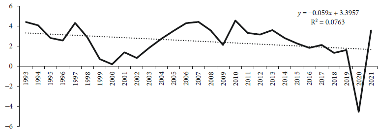
The graphic of the autonomous total GDP by period, resulting from the OLSTDV model, is presented in Figure 1. As it is shown, the time intercepts do not follow a systematic trend over time (only a marginal decreasing trend is captured); instead, they follow a cyclical pattern associated to economic downturns or economic crisis as those of 1995, 2000, 2009 and 2020. In contrast, in the companion paper it was found that the autonomous total GDP of the European countries’ sample follows a clearer decreasing trend over time, explained mainly by deindustrialisation.

Note: P value of F test (0.000).
Source: Own computation.
Figure 1 Autonomous total GDP growth, obtained from equation [2] OLSTDV
The outcome resulted from the first Kaldor’s law represented in equation [3] is illustrated in Table 2. The F and the BPLM test from the FE and RE models respectively indicate the presence of country effects, but at 90% of statistical significance, while the Hausman tests rejects the null H0: difference in coefficients not systematic; the FE model is therefore the preferred specification.
Table 2 Equation [3], first Kaldor’s law
| OLS (1) | Fixed effects (2) |
Random effects (3) |
GMMDIF (4) |
|
|---|---|---|---|---|
| GDPgnonmant-1 | 0.214 | |||
| GDPgman | 0.557* | 0.544* | 0.553* | 0.589 |
| Constant | 2.103* | 2.136* | 2.111* | 1.236 |
| R2 | 0.512 | 0.513 | 0.513 | |
| F | (0.056) | |||
| BPLM | (0.072) | |||
| Hausman | (0.007) | |||
| DWM | 1.534 | |||
| Baltagi-Wu | 1.626 | |||
| AR(1) | ||||
| AR(2) | ||||
| AR(3) | ||||
| Sargan | (0.455) |
Notes: The dependent variable is the non-manufacturing GDP rate of growth. (*p < 0.01, **p < 0.05, ***p < 0.10). P value in parenthesis. 348 observations.
Source: Own computation.
According to the FE coefficients presented in column 2, an increase of one percentage point in the explanatory variable (GDPgman) is associated to a rise of 0.544 percentage points in non-manufacturing GDP growth (GDPgnonman), and the autonomous dependent variable is 2.136 percent, which represents a substantial and contemporary autonomy of the non-manufacturing GDP growth from the total GDP. The slope coefficient for the case of Europe is lower (0.367) and the constant is nearly zero; these figures show that in Europe the effect of the manufacturing GDP growth on the non-manufacturing GDP growth is smaller than in Latin America, and the non-manufacturing GDP fully depends on the manufacturing GDP.
By disaggregating the explanatory variable’s slope in the three country classifications we find that the slope for the high manufacturing employment countries is 0.590, for the middle manufacturing employment countries is 0.583, and for the low manufacturing employment countries is 0.443. Hence, there is a positive relationship between the effect of manufacturing GDP growth on non-manufacturing employment growth with the share of manufacturing employment to total employment; while in the companion paper it is shown that deindustrialisation is inversely associated to the growth of non-manufacturing GDP.
The coefficient on manufacturing GDP growth goes from 0.544 in the fixed effect model to 0.589 in the dynamic model; the coefficient increases 0.45. In turn, column 4 shows a dynamic effect in which a growth of 1 percent in contemporaneous non-manufacturing GDP is associated with a growth of 0.214 percent of the variable in a later period. That is to say, non-manufacturing GDP growth comes from its own lag and from manufacturing GDP.
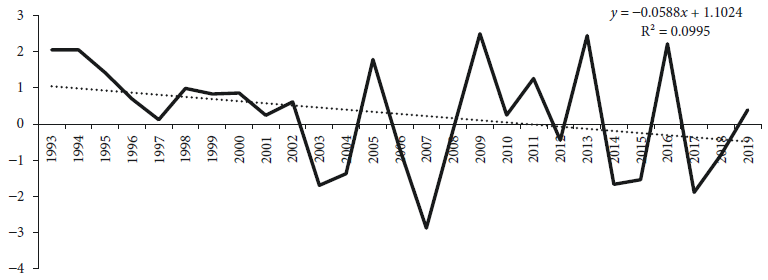
Figure 2 illustrates the trend of the autonomous non-manufacturing GDP growth by period, resulting from the OLSTDV model. The time intercepts do not follow a clear decreasing trend over time, as do the sample of European countries in the companion paper; instead, they follow a cyclical pattern associated to economic downturns or crisis.
Note: P value of F test (0.000).
Source: Own computation.
Figure 2 Autonomous non-manufacturing GDP growth, obtained from equation [3] OLSTDV
The estimations from the first Kaldor’s law in equation [4] are presented in Table 3. The F test and the BPLM tests conducted in the FE and RE model respectively do not capture the presence of country-specific effects, in this case the OLS model is preferred. An upturn of one percentage point in the non-manufacturing GDP growth is associated to a nearly one to one increase in the total GDP growth (0.985). This result is in keeping with those obtained from the original Kaldor study and the companion paper study on European countries, which find a coefficient around one.
Table 3 Equation [4], first Kaldor’s law
| OLS (1) | Fixed effects (2) |
Random effects (3) |
GMMSYS (4) |
|
|---|---|---|---|---|
| GDPgtott-1 | -0.039* | |||
| GDPgnonman | 0.985* | 0.987* | 0.985* | 0.997* |
| Constant | -0.107* | -0.112* | -0.107* | -0.011 |
| R2 | 0.980 | 0.980 | 0.980 | |
| F | (0.724) | |||
| BPLM | (0.998) | |||
| Hausman | (0.464) | |||
| DWM | 1.666 | |||
| Baltagi-Wu | 1.825 | |||
| AR(1) | (0.033) | |||
| AR(2) | (0.840) | |||
| AR(3) | (0.826) | |||
| Sargan | (0.102) |
Notes: The dependent variable is the total GDP rate of growth. (*p < 0.01, **p < 0.05, ***p < 0.10). P value in parenthesis. 348 observations.
Source: Own computation.
When the non-manufacturing GDP growth slope coefficient is disaggregated by countries, all the country coefficients approximate one; moreover, the country group classification shows that the slope in high industrial employment is 0.996, in middle industrial employment countries is 0.978, and in low industrial employment countries is 0.972, indicating a small variation among them. This fact points out that the relationship between non-manufacturing GDP growth and total GDP growth is relatively constant both in European and Latin American countries and it approximates a one-to-one coefficient.
The intercept coefficient in the OLS model in Table 3 is small (-0.107) and the magnitude is even smaller for the case of European countries, which suggests that the variables in the model, non-manufacturing GDP growth and total GDP growth are not mutually autonomous and have strong contemporaneous dependency. It should be noted that in the static model (column 2) there is no evidence of autocorrelation, and to some extent this is consistent with the dynamic model, because the lagged dependent variable, although statistically significant, its magnitude is negative and small (-0.039), compared to the previous models. This finding suggests that the non-manufacturing GDP growth produces a small and reversive dynamic effect on the total GDP growth. In other words, the relationship between the two variables is mainly contemporaneous and not dynamic.
The total GDP growth, autonomous from the non-manufacturing GDP growth, is low (between -0.33 and 0.56 percent) over time, and does not present a systemic trend; as in the previous models, is mainly cyclical in relation to crisis o recession periods. The result suggests that total GDP growth has a strong dependence on economic cyclicality and on non-manufacturing GDP, but the latter is unable to transmit a substantial and dynamic economic growth effect.

Note: P value of F test (0.008).
Source: Own computation.
Figure 3 Autonomous total GDP growth, obtained from equation [4] OLSTDV
The estimation of the second Kaldor’s law in equation [5] rejects the null hypothesis ‘no specific effects across countries’ both in the FE and RE specifications, by conducting the F and BPLM tests respectively. Consequently, the OLS model is not convenient. The Hausman test does not reject the null hypothesis ‘difference in coefficients not systematic’, thus, both models FE and RE are consistent. We use the FE model for interpretations.
An increase of one percentage point in manufacturing GDP growth leads to a rise of 0.335 percentage points in the manufacturing labour productivity (MLP), this coefficient is low, nearly half of that obtained in the companion paper (0.656) for the case of European countries, and even smaller than that obtained by Kaldor (0.50). This finding points out that manufacturing GDP growth is less effective to generate manufacturing productivity in Latin America than in Europe.
When the coefficient on manufacturing GDP growth is disaggregated by the three country groups classification, by applying the OLSSDV, we find that the coefficient for high manufacturing employment is 0.347, for middle manufacturing employment is 0.311, and for low manufacturing employment is 0.384. This outcome indicates that there is not a systematic trend between the level of manufacturing employment and the impact of manufacturing GDP growth on the growth of manufacturing labour productivity. In contrast, for the European countries case there is a positive relationship between the level of deindustrialisation and the effect of manufacturing GDP growth on manufacturing labour productivity.
Although the coefficient on manufacturing GDP growth is relatively low in the statistical specifications, the dynamic mechanism in the equation is relevant, as the coefficient of the lagged dependent variable is 0.200, while in the European country sample is even negative (-0.081) and smaller. The intercept in the FE equation is 0.420 and in the companion paper is close to cero (0.016); this finding illustrates that manufacturing labour productivity is less dependent on manufacturing GDP growth in Latin America than in Europe, but the relationship between the two variables fosters a dynamic process in MLP in Latin America.
Table 4 Equation [5], second Kaldor’s law
| OLS (1) | Fixed effects (2) |
Random effects (3) |
GMMSYS (4) |
|
|---|---|---|---|---|
| MLPgt-1 | 0.200* | |||
| GDPgman | 0.350* | 0.335* | 0.343* | 0.501* |
| Constant | 0.383 | 0.420 | 0.401 | -0.292 |
| R2 | 0.107 | 0.107 | 0.107 | |
| F | (0.032) | |||
| BPLM | (0.031) | |||
| Hausman | (0.404) | |||
| DWM | 1.901 | |||
| Baltagi-Wu | 1.955 | |||
| AR(1) | (0.000) | |||
| AR(2) | (0.025) | |||
| AR(3) | (0.228) | |||
| Sargan | (0.156) |
Notes: The dependent variable is the manufacturing labour productivity rate of growth. (*p < 0.01, **p < 0.05, ***p < 0.10). P value in parenthesis. 324 observations.
Source: Own computation.
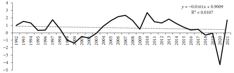
The graphic of time intercepts is presented in Figure 4, it is appreciated that autonomous manufacturing labour productivity does not follow a clear systematic trend over the years, not even in relation to economic downturns. If we adjust a trend line, it can be seen there is a marginal decreasing trend. In contrast, the European countries present an increasing trend over time. This outcome shows that autonomous MLP is stagnant in the Latin American countries sample and is even slightly regressive, contrary to the trend in the European countries sample, where autonomous manufacturing labour productivity increases despite deindustrialisation.
Note: P value of F test (0.510).
Source: Own computation.
Figure 4 Autonomous manufacturing labour productivity growth, obtained from equation [5] OLSTDV
The estimations from the third Kaldor’s law (equation [8]) are presented in Table 5. Both the F and BPLM test reject the null hypothesis of no country-specific effects in the FE and RE specifications respectively. The Hausman test validates the null hypothesis of ‘difference in coefficients not systematic’; therefore, both estimations, FE and RE are consistent. We take FE for interpretations.
Table 5 Equation [8], third Kaldor’s law
| OLS (1) | Fixed effects (2) |
Random effects (3) |
GMMDIF (4) |
|
|---|---|---|---|---|
| TLPgt-1 | 0.175* | |||
| GDPgman | 0.528* | 0.519* | 0.523* | 0.550* |
| NMEG | 0.226* | 0.243* | 0.235* | 0.224* |
| Constant | 0.095 | 0.072 | 0.083 | -0.292** |
| R2 | 0.676 | 0.675 | ||
| F | (0.000) | |||
| BPLM | (0.000) | |||
| Hausman | (0.205) | |||
| DWM | 1.441 | |||
| Baltagi-Wu | 1.514 | |||
| AR(1) | (0.019) | |||
| AR(2) | (0.509) | |||
| AR(3) | (0.735) | |||
| Sargan | (0.097) |
Notes: The dependent variable is the total labour productivity rate of growth. (*p < 0.01, **p < 0.05, ***p < 0.10). P value in parenthesis. 360 observations.
Source: Own computation.
An increase of one percentage point in manufacturing GDP growth (GDPgman) leads to a rise of 0.519 percentage points in total labour productivity growth (TLPg), the magnitude of the effect is smaller than that obtained in the companion paper (0.728). This outcome shows that the contribution of manufacturing growth to total labour productivity is smaller in Latin America than in Europe. The disaggregation of the coefficient by the country’s classification shows a positive relationship between the level of manufacturing employment and the effect of manufacturing GDP growth on total labour productivity. The coefficient is 0.562 for high manufacturing employment countries, 0.525 for the middle manufacturing employment’s classification, and 0.401 for low manufacturing employment countries. In the European case, there is not a systematic relationship between the coefficient and the level of deindustrialisation.
What is striking is the coefficient on non-manufacturing employment growth, as it enters equation [8] with a positive sign, while in the Kaldorian postulates the coefficient is expected to be negative. An upturn of one percentage point in non-manufacturing employment growth (NMEG) leads to a rise of 0.243 percentage points in total labour productivity growth; in contrast, the coefficient is -0.590 for the European country sample in the companion paper, in line with Kaldor’s original estimation.
By disaggregating the coefficient across the classification of countries, it is found a direct relationship between the level of manufacturing employment and the effect of non-manufacturing employment growth on total labour productivity growth, an upturn of one percentage point in non-manufacturing employment growth leads to an increase in total labour productivity of 0.363 percentage point in high manufacturing employment countries, 0.258 in middle countries, and 0.217 in low countries, while in the sample of European countries a rise in non-manufacturing employment growth reduces more total labour productivity on countries with more deindustrialisation.
The intercept is not statistically significant neither in the Latin American sample nor in the European sample. The dynamic equation in column 4 shows an increase of 0.175 percentage point in the current period due to a rise of one percentage point in the previous period. There is a larger coefficient of manufacturing GDP growth and a smaller coefficient of non-manufacturing employment growth compared to the static specification, and the intercept becomes negative.
The autonomous total labour productivity growth oscillates with the economic downturns, but in the long run does not show a clear systematic pattern, it rather remains steady. In contrast, in the European countries sample the intercepts follow a decreasing trend.
5. CONCLUSIONS
2023 marks four decades of Thirlwall’s seminal work “A Plain Man’s Guide to Kaldor’s Growth Laws”, in which the contributions of Nicholas Kaldor (1966) are discussed in relation to the role of the manufacturing sector in economic growth. This paper highlights the role of manufacturing GDP growth in total GDP growth, through what has come to be known as the Kaldor-Verdoorn Laws, which have their theoretical background in the works by Smith, Ricardo, and Young.
The changes that occurred in the forty years after the publication of Thirlwall’s work make it necessary to reassess the applicability of these laws in the context of economic opening and globalization. These led to the expansion of markets and the distribution of production at a global level, being the developing economies in particular the ones that applied deep reforms with the purpose of consolidating the expansion of markets, through the increase of their exports.
The econometric results in this paper demonstrate compliance with the Thirlwall-Verdoorn Laws for the sample of twelve Latin American countries, with some particularities. First, there is the presence of a positive effect of the growth of production in the manufacturing sector on total GDP growth, higher than that found in European economies. This indicates the presence of a manufacturing sector with a high traction capacity and dynamic effects on the rest of the economic sectors.
Second, the increase in manufacturing production is directly related to the increase in productivity, although it stands out that its effect is less compared to that found for European countries by Ángeles, Fraga, and Domínguez (2019). This result, at least in part, is explained by the lower specialization in the production of high value-added goods in the Latin American economies.
Third, it is also worth noting that the manufacturing sector boosts a dynamic effect on its productivity, this result is not found for the European economies; hence, although the manufacturing sector has a smaller effect on its productivity in Latin America, it has the capacity to foster a dynamic effect on manufacturing labour productivity.
Finally, the positive influence of the increase in manufacturing production on total productivity is also accompanied by a positive effect of non-manufacturing employment on productivity. This result stands out for being different from the one found by Kaldor and the case of European countries, although it can be explained by the presence of high levels of underemployment and informality, which prevents the transfer of formal workers from other sectors of the economy.
Based on these results, it is important that governments consider the design and implementation of industrial policies that lead to the production of goods with higher added value in the Latin American economies, which will allow the relaxation of external restrictions on growth, a broad desire of the Latin American countries. This should be a priority objective for governments, since as Thirlwall (2003) points out, industrialisation is an objective that often requires public policies, as evidenced by the cases of South Korea and China, among others. In other words, industrialisation is not a spontaneous result of the market, and industrialisation policies are even more necessary in an environment of greater global competition.

