


 nueva página del texto (beta)
 Inglés (pdf)
 Artículo en XML
 Referencias del artículo
 Enviar artículo por email
 Citado por SciELO
  Similares en
SciELO
Similares en
SciELO 
 Permalink
1. INTRODUCTION
The greater importance of income distribution as a central element in the dynamics of economic growth has been formally presented since the beginning of the development of the Cambridge school’s growth and distribution models. Those developed by Kaldor (1956, 1957) and Pasinetti (1962) aim to solve the problem of the “razor’s edge” arising Harrod’s model (1939).
Income distribution was also present early on in Prebisch (1949), Furtado (1980 [1959]) and Medina (1963). However, with the work of Fajnzylberg (2000) and a series of studies sponsored by the Economic Commission for Latin America and the Caribbean (ECLAC), such as ECLAC (1990, 1992a, 1992b, 1993, 1997), this concern took its place as a central object of interest.
This emphasis on the role of income distribution in economic development is because there is practically no significant correlation between the process of economic development and income concentration when analyzing extended periods of development (Piketty, 2014). Empirical evidence, as in Park (1996) and Hein and Vogel (2008), suggests that greater social equity provides, through various channels (such as greater human capital and social stability), economic development.
The goal of this work is to present an economic growth model with a balance of payments constraint, in which income distribution and the technological gap play central roles in determining the pace of technological progress in a developing economy1. Therefore, the model embodies different possible patterns of development based on the role played by income distribution, which is an inseparable element of the catching up process toward a more equitable and dynamic economy.
There are two economies -the North and the South- whose main difference between them is the existence of asymmetries in the stock of knowledge, with the North being on the technological frontier. Furthermore, the South has a productive structure characterized by the production of low-income elasticity demand of goods.
Both economies produce a single good usable for consumption and investment. The South has a constant product-capital ratio and an oligopolistic market structure. It is further assumed that the South is a small open economy, so its actions do not affect prices, wages, or the pace of technological progress in the North.
In this framework, four possible economic growth patterns for the South economy are presented, following Fajnzylberg (2000): 1) dynamic and disarticulated, i.e., with a high rate of economic growth but high income inequality; 2) integrated and stagnant, in other words, with a low economic growth rate but high income distribution; 3) disarticulated and stagnant, i.e., with a low rate of economic growth and income distribution; and, finally, 4) dynamic with social equity, in other words, with a high rate of economic growth and, also, with wide income distribution. To the best of our knowledge, there is no balance of payment constrained growth model (BPCG) that explores these four possible patterns according to Fajnzylberg’s (2000) arguments about economic development in a North-South framework.
The North-South models of Cimoli (1988), Dutt (2003), and Blecker (1996), as well as Skott and Larudee (1998), Ros and Skott (1997), Porcile and Cimoli (2007), Ros (2000), Botta (2009, 2012) and Gabriel, Jayme JR, and Oreiro (2016) are examples of this tradition. The common feature of them is the role of productive and trade asymmetries between developed and developing countries as well as the balance of payments disequilibrium in a demand-led economic growth model.
The present study is structured into five additional sections. In Section 2, the structure of the model is presented through four blocks. Then, in Section 3, the dynamics of income distribution and technological progress are presented. Then, in Section 4, the various possibilities for economic growth patterns in a BPCG scenario are analyzed. In Section 5, a series of comparative dynamics analyses are carried out to investigate the role of some key variables in the model. Finally, in Section 6, the main conclusions of the study are presented.
2. MODEL STRUCTURE
One of the ECLAC’s leading researchers was Fernando Fajnzylberg. According to Bielschowsky (2009) he argued that both social equity (i.e., better income distribution) and technical progress (i.e., lower technological gap) were important to increasing competitiveness. However, this competitiveness should be “authentic,” and should be based on the increasing implementation of new technologies and new human capital skills, while “spurious” competitiveness measures based on low wages and natural resources should be avoided (Fajnzylberg, 1988).
In the next section we present the BPCG model that will explore four possible patterns according to Fajnzylberg’s (2000) arguments about economic development that helps explaining Latin American economies according to theoretical framework in a North and South modelling.
2.1. Balance of payment constrained growth
The process of long-term economic growth in the South is restricted by the availability of foreign exchange from its exports. Furthermore, the South is a small open economy whose action does not affect the North’s economy, so its imports depend only on the nominal exchange rate and its real income level. So:
Where M represents the South’s imports (in terms of quantum), P* is the price level from the North, P is the price level from the South, E is the nominal exchange rate, Y is the real income from the South and Ψ and π are imports price elasticity and imports income elasticity, respectively.
Exports (in terms of quantum) from the South depend on three factors, the nominal exchange rate, the income of the North and, following Amable (1994) and Porcile, Dutra, and Meirelles (2007), an export quality index. Therefore, it follows that:
Where X represents exports, Z is real income from the North, Ω represents a quality index from South exports2, and η and ε are export price elasticity and export income elasticity, respectively. Furthermore, λ is the export quality elasticity.
The equilibrium condition in the balance of payments in the absence of capital flows is:
The export quality index depends directly on the inverse of the technological gap between North and South (S), so that the rate of change of the export quality index (ω) increases, according to the sensitivity coefficient (ϖ). In this way:
The inverse of the technological gap is defined as the ratio of the South’s stock of knowledge to that of the North. As the North is ahead of the South in terms of knowledge, it follows that 0 < S ≤ 1. Then,
Where T S is the South stock of knowledge and T N is the North stock of knowledge.
Substituting equations [1] and [2] into [3] and puting the result of this substitution in terms of the rate of change, the following is obtained:
In equation [6], the lowercase letters represent the rate of change of the variable in question. Assuming that the purchasing power parity principle (PPP) prevails in the long run (p - p* - e = 0) substituting equation [4] into [6], it follows that:
Where it was assumed, without loss of generality, that ϖ = 1.
Equation [7] presents the South growth rate compatible with equilibrium in the balance of payments, which depends on the growth rate of external income, z, and the income export elasticity as well as the inverse of the technological gap, S, and the export quality elasticity, λ. Both variables are weighted by import income elasticity.
Therefore, equation [7] is Thirlwall’s Law with the inclusion of a new argument that captures the technological difference between the South and the North (inverse of the technological gap), as well as the quality of southern exports.
2.2. Production and functional distribution of income
As only one good is produced, and it is used either for consumption or for investment and as there are only two factors of production -capital and labor- it follows that the production of the South can be described by the following fixed coefficient function:
Where K is the South capital stock, u K represents the potential output-capital stock ratio, L is the employment level and a S is the output-labor ratio of the South (a S = Y/L).
Southern oligopolistic firms operate to meet demand, which, in turn, is always below potential production, so that there is excess production capacity at any given time. Furthermore, as firms do not have long-term contracts with the workforce and do not incur the costs of hiring, training and firing workers, they hire labor to the exact extent of their needs. Thus, it follows that the level of employment in the South (L) is determined by its level of production:
The existence of idle capacity in the production process is a characteristic of modern capitalist economies. Several arguments can be put forward to justify the existence of idleness in productive capacity. Following Steindl’s (1952) argument, firms reserve a certain idle capacity to retaliate with an increase in production (and consequent fall in prices and profits) to an eventual rival firm. Otherwise, a certain idle capacity is necessary to respond promptly to unexpected changes in demand, since “producers can’t know what consumers will want to buy in the future because consumers themselves don’t know” (Kregel, 1980, p. 37).
Following the works of Kaldor (1956), Kalecki (1971), Pasinetti (1962), Robinson (1956, 1981 [1962]), Rowthorn (1980) and Taylor (1985), among others, the economy of the South is composed of two social classes -capitalists and workers- that differ from each other according to the origin of their income, profits and wages, respectively. In effect, the real income of the South is divided between these two classes as follows:
Where V = W/P represents the real wage in the South.
As the market structure of the South is characterized by the existence of oligopolistic firms, they have some market power such that their prices are determined by a mark-up rate on the unit costs of production:
Where (( is the South mark-up rate. Dividing equation [10] by the capital stock, it follows that the rate of profit is:
Where r is the profit rate in the South, defined as the monetary flow of profits divided by the stock of capital, and u is the degree of capacity utilization (u = Y/K)3.
The share of profits in income is the difference between real income and the share of wages in income, since there are only two social classes:
Where m is the profit share in the South (0 < m < 1), and ( is the wage share in the South (0 < ( < 1)4. Both shares in terms of South’s income.
Substituting equations [9] and [12] into [10], we have the wage share:
Manipulating equation [11] algebraically, it is possible to show that the share of wages in income depends only on the firms’ markup rate.
Using equation [15] in equation [14] shows that the share of profits in income also depends only on the firms’ markup rate:
Equations [15] and [16] indicate that the higher the mark-up rate is, the greater the share of profits in income. In the limiting case where the mark-up rate tends to infinity, the share of profits (wages) in income will tend to one (zero). Conversely, if the mark-up rate tends to zero, the share of profits (wages) in income will tend to zero (one).
2.3. Technological innovation process
The stock of knowledge in the South is fundamentally affected by the degree of income distribution. According to Ros (2013) the effects of income distribution on technological change and growth depend crucially on whether technological change takes place in the modern tradable sector or in the subsistence sector. If it takes place in the former, the greater the elasticity of the quality of exports, productivity, the higher skilled workers and wages when compared to the latter. It is in the modern tradable sector where the South economy has greater stock of knowledge. Moreover, we assume that the South’s stock of knowledge rises when the technological gap narrows.
Where circumflex over T S is the stock of knowledge rate of growth of the South, α represents the sensitivity of the technical progress in relation to income distribution (0 < α < 1), and β is the sensitivity coefficient of the technical progress in relation to the inverse of the technological gap. Furthermore, 0 < β < 1 and the greater the stock of knowledge of the South is, the greater the technological progress.
When income distribution is excessively concentrated with capitalists or workers, the stock of knowledge of the South tends to be low. On the one hand, when income mostly concentrates with capitalists, there are few incentives to invest in modern technologies (e.g., by research and development) because there is low potential for future consumption in the domestic market and a low level of competitiveness with the North, which is at the frontier of knowledge. On the other hand, when the income is excessively concentrated with workers, there are incentives to consume more. However, capitalists do not have enough resources to invest in new technologies, although they have incentives with consumers. Therefore, only for intermediate levels of the wage share (σ1 < σ < σ2) there is a combination of incentives and capabilities so that an intensification of the rate of technological innovation occurs.
The first channel of the intermediate range of σ in the South economy comes from the benefits from greater social cohesion, resulting from less inequality between capitalists and workers, which will allow the latter to withstand more pronounced social and technological changes (Fajnzylberg, 2000). The second channel of influence arises when the wage share is seen from a broader point of view, as representing greater access to public health and education by workers (Porcile, Dutra, and Meirelles, 2007).
The rise in the productivity growth rate of the South increases with the growth of the stock of knowledge:
Where a S with circumflex represents the growth rate of labor productivity.
The North’s stock of knowledge grows from the following function:
Where T N with circumflex is the Northern knowledge growth rate, τ0 is a positive parameter that captures the autonomous growth of Northern knowledge and τ1 is the sensitivity coefficient of the inverse of the technological gap; the smaller it is the faster the technology gap will narrow.
The stock of knowledge rate of growth in equations [18] and [19] refers to the productive knowledge growth in the economy. It is easier for countries to produce new goods or provide new services from the knowledge they developed as long as this means adding a new productive process in the economy. This process depends on the social accumulation of productive knowledge (Verspagen, 1993; Hausmann et al., 2011).
2.4. The labor market
The labor market of the South is permeated by the distributive conflict between capitalists and workers. Thus, the nominal wage growth rate will increase whenever the wage share desired by workers is greater than the effective wage share (Lima, 2002). Therefore, it follows that:
Where V with circumflex is the nominal wage growth rate, σ V is the wage share desired by workers and φ is the sensibility coefficient greater than zero and smaller than one.
Assuming that prices in the South, as well as prices in the North, are fixed both in the short and in the long run, it becomes possible to carry out the subsequent analysis, highlighting the distributive conflict present in the labor market and the process of technological development of the South.
The wage share desired by workers depends on the rate of employment growth and the bargaining power of workers. Thus, whenever the labor market shows an upward trend in job demand, workers will be in a better position to claim a higher salary share, as follows:
Where ξ with circumflex represents the employment rate variation, γ represents the bargaining power of workers (0 < γ < 1), and ξ (without circumflex) represents the employment rate, which is the employment of the South (L) and the supply of work (N), i.e., ξ = L/N.
Given the definition of the employment rate, it follows that the rate of change of employment in the South is:
Where L with circumflex is the demand growth rate of employment (demand) and N with circumflex is the supply growth rate of employment of the South.
The growth rate of the labor supply is assumed to be constant:
Where n with slash is the constant growth rate of the labor supply.
3. THE DYNAMICS OF INCOME DISTRIBUTION AND THE TECHNOLOGICAL GAP
Substituting equations [22] and [23] into equation [21] and the resultant into equation [20], it is possible to determine the equation that describes the growth rate of the nominal wage over time as a function of the exogenous growth rate of the labor supply, the share of wages in income and the growth rate of the employment level of the South, as shown below:
By linearizing and deriving equation [9] with respect to time, it is possible to determine the growth rate of the employment level in the South as follows:
Finally, using equations [7], [17], [18] and [25] in equation [24], we have:
Where it was assumed for simplification that φ = 1 and defined the new parameters as follows:
Equation [26] describes the wage growth rate as a nonlinear function of the share of wages in income and as a direct function of the inverse of the technology gap (S).
The condition for an increase in the inverse of the technological gap to cause an increase in the growth rate of nominal wages is λ/π > β. In other words, it is necessary that the ratio between the elasticity of the quality of exports in relation to the income elasticity of imports is greater than the influence of the level of the inverse of the technological gap on the rate of technological progress in the South.
Linearizing equation [14] and deriving it with respect to time, it follows that:
Where σ with circumflex is the rate of change of the wage share in income.
By substituting equation [17] into [18] and the equation resulting from that substitution, together with equation [26], into [27], we arrive at the equation that describes the dynamics of the wage share compatible with the balance of payments equilibrium:
Where the parameters are defined as follows:
For ρ0 > 0, it is necessary that the product of the income elasticities of exports and imports with the growth rate of income in the North is greater than the value of the growth rate of labor supply5.
Additionally, we assume that ρ3 > 0. This assumption is true if the sensitivity of the growth rate of knowledge in the South is relatively small when compared with the bargaining power of workers and the ratio between the elasticities of export quality and import income. Finally, ρ1 > 0 and ρ2 > 0 are straightforward.
The equation that describes the combinations between the inverse of the technological gap and the wage share for which the wage share remains constant over time, that is, the equation that describes the locus σ with circumflex equals to 0 is:
Equation [29] shows that in plane (S - σ), the locus σ (with circumflex) is a parabola with a negative intercept, which is equal to (-ρ0/ρ3) and with the concavity facing downward6. Moreover, the maximum point of this parabola corresponds to the following level of the wage share: ρ1/2ρ2.
The necessary and sufficient conditions for ∂S/∂σ > 0 in the first and second regions are ∂S/∂σ < 0, and those in the third region are σ* < ρ1/2ρ2 and σ** > ρ1/2ρ2, respectively. That is, there must be two regions in plane (S - σ) divided by a separatrix that cuts locus σ (with circumflex) at its maximum point.
Given the quadratic relationship between locus σ (with circumflex) and wage share, there can be up to two real roots in space (k - σ). However, only one of them is in the economically relevant space. Figure 1 illustrates the discussed locus under the assumptions made7.

Equation [5] describes the inverse of the technological gap; linearizing and deriving it with respect to time, we have:
Using equations [17] and [19] in equation [30], the equation that describes the dynamics over time of the inverse of the technological gap is:
As the equation above shows, the rate of change of the inverse of the technology gap depends nonlinearly on the wage share and inversely on the level of the inverse of the technology gap.
The combinations of the inverse of the technology gap and the share of wages in income for which the rate of change of the inverse of the technology gap is equal to zero, that is, the equation that describes the locus Ŝ = 0 is:
As we assume that the reaction of technological progress in the North is greater than the reaction of technological progress in the South with respect to reductions in the technological gap, that is, that τ1 > β, it follows that locus Ŝ = 0 has a negative intercept equal to [-τ0/(τ1 - β)]. The analysis of locus Ŝ = 0 also shows that it has two real roots in the economically relevant space and that it is a parabola with the concavity facing downward and with a maximum point. Figure 2 depicts this case8.

4. ANALYSIS OF EQUILIBRIUM CONDITIONS
The long-run equilibrium analysis between the inverse of the technology gap, S, and wage share, σ, can be obtained using equations [28] and [31]. Returning to these two equations, it follows that:
Therefore, we have a two-dimensional nonlinear system of differential equations that describe the dynamics over time of the inverse of the technological gap and the wage share. Due to the parametric constraints presented earlier, plane (S - σ) can be disassembled into three regions that are divided by two separatrices (shown in Figure 3, below). Therefore, the (S - σ) plane is divided into three regions according to the slope of the loci. These regions are called I, II and III.

It is worth mentioning that the assumption that the sensitivity of technological progress in the North with respect to the technological gap is greater than its equivalent for the economy of the South, that is, τ1 > β, is fundamental both to determine the slope of the locus Ŝ = 0 regarding the conditions for the existence of one or more equilibria as well as the stability of the system.
Indeed, if β > τ1, then above-mentioned locus will have a positive intercept, and its concavity will turn upward. Thus, denoting a negative slope for region I and a positive slope for regions I and II. The system would then present two equilibrium points, one in region I and the other at some point in region III, whose stabilities would be stable and unstable, respectively.
Therefore, the condition of the relative weight of these two technological parameters is of fundamental importance to, for example, determine whether equilibrium will be found in regions with a high-income distribution. It is even more interesting to note that if β > τ1, then the stability zone will occur in region I, characterized by a low-income distribution.
Due to the way in which the wage share was defined and the inverse of the technological gap, plane (S - σ) is between zero and one. As this space is an economically relevant area, any segment of any of the loci that exceeds these limitations has no economic significance and, therefore, is not considered in the analysis.
Thus, locus Ŝ = 0 is a parabola with the concavity facing downward and with two positive roots between zero and one. Furthermore, there is a maximum point of this isocline (see Figure 3).
The locus σ (with circumflex) has a negative intercept and describes a parabola with the concavity facing downward. Furthermore, it has two real roots, but only one of them assumes values between zero and one. Moreover, there is a maximum point (see Figure 3).
The matrix of partial derivatives of this nonlinear two-dimensional system is:
The elements J12 and J22 of this Jacobian matrix present positive and negative signs for any value of the wage share and the inverse of the technological gap, respectively. Thus, the equilibrium of this nonlinear dynamic system depends on the values assumed by the elements J11 and J21.
Since the maximum point of locus σ (with circumflex) is necessarily to the right of the maximum point of locus Ŝ = 0 and to the left of the maximum point of locus σ (with circumflex), it follows that elements J11 and J22 both assume negative signs. Thus, the Jacobian matrix of partial derivatives for the region around the equilibrium (point E) is as follows:
Thus, this matrix unambiguously presents a trace smaller than zero and in the case J11J22 > J21J12 a positive determinant. Thus, it presents a stable focus characterized by damped spirals at the equilibrium point E. On the other hand, if we consider that the locus Ŝ = 0 crosses the locus σ (with circumflex) at the maximum point of the latter, then the Poincaré-Bendixson theorem would ensure the presence of a stable limit cycle in E (De La Fuente, 2000)9.
With reference to the above discussion, Figure 3 illustrates the situation in which there is a stable equilibrium characterized by damped spirals at E. Thus, a trajectory that leaves, for example, point A, will present a dynamic characterized by damped spirals until reaching equilibrium point E. Therefore, the system presents a large zone of stability around the stable focus.
5. COMPARATIVE DYNAMICS ANALYSIS
Once the conditions have been defined for the system to present the characteristics described in the previous section, carrying out some comparative dynamics analysis it is possible to better understand how the inverse of the technological gap and the wage share changes in some of the model parameters.
To be able to associate the effects of the parametric changes that will be carried out below on the growth rate of the South, it is first necessary to define the influence that the inverse of the technological gap has on the economic growth of the South. Returning to equation [7], which describes the growth rate of the South compatible with the balance of payments equilibrium, we have:
Therefore, it follows that the influence of the inverse of the technological gap on the growth rate of the South is:
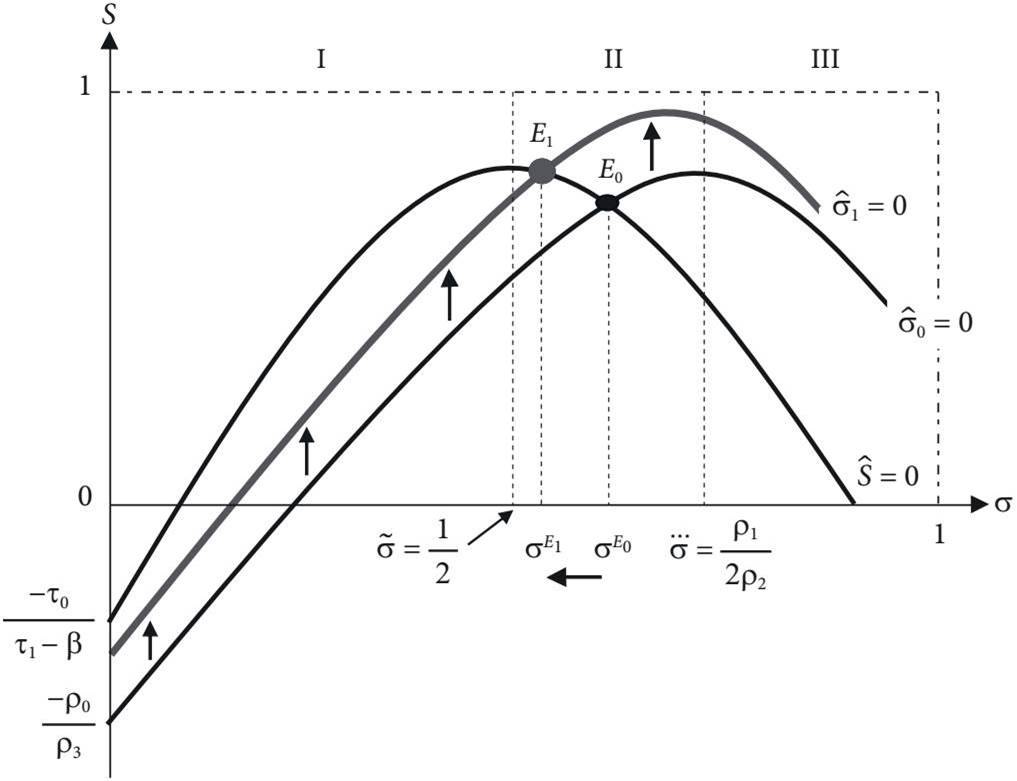
The increase in the relative growth rate of technological progress in the North with respect to the South, as shown in Figure 4, increases the difference between the North and South’s technology gap if the wage share is low. On the other hand, if the wage share is high, the difference between the technological gap between the North and the South will decrease and the income distribution of the South will improve (i.e., increase in the wage share).
The derivative that describes the influence of the relative difference between the sensitivity of North and South technological progress is10:

As (τ1 - β) belongs only to the Ŝ = 0 locus argument, it follows that increasing the relative sensitivity between North and South technological progress, (τ1 - β) shifts the locus up in region I and up in regions II and III. Furthermore, since the inverse of the technological gap rises around equilibrium, it follows that the growth rate of the economy of the South increases with the acceleration of technological progress in the North. As shown below:
In fact, the relative increase in the expansion of technological progress in the North vis-à-vis the South leads to an increase in growth at the same time that it increases the distribution of income in favor of workers, which shows the possibility of reconciling a growth process with social equity.
The analysis of the increase in the South’s labor supply on its growth and income distribution can be easily done. Recalling that the labor supply of the South is part of the locus argument σ (with circumflex) only and belongs to the parameter ρ0, it follows that its change affects the intercept of this locus directly. Thus, we have that the inverse derivative of the technological gap with respect to the labor supply is:
Therefore, the effect of the increase in labor supply on growth will also be positive, as presented below:
Therefore, the increase in the South’s labor supply raises the inverse of the technological gap and, consequently, the South’s income growth rate (as shown in Figure 5). However, it decreases the income distribution in favor of workers (i.e., the wage share is lower). Thus, a growth process compatible with a dynamic economy, but disjointed.
Regarding the effect of the influence of income distribution on technological progress in the South, coefficient α affects both locus σ (with circumflex) and locus Ŝ = 0 since it is part of the arguments of parameters ρ1 and σ2. That said, we have that the effect of increasing this coefficient on the technological gap for σ (with circumflex) > 0 loci and Ŝ > 0 is, respectively:
This implies an increase in the income growth rate of the South:
As evidenced by the equations above and by Figure 6 both locus σ (with circumflex) > 0 and Ŝ > 0 shift upward due to the increase in coefficient α. Furthermore, as the effect on the inverse of the technological gap is greater for locus Ŝ > 0, it follows that the net effect of increasing this coefficient on income distribution is to increase it in favor of workers. Thus, this process characterizes a development process with high economic growth and social equity.

The impact of an increase in income in the North on the economy of the South can be verified by the following derivative:
Therefore, the impact of an increase in Northern income on Southern income will be:
Since the income of the North is only part of the argument of the parameter ρ0, it follows that its intercept is affected, being shifted downward, as shown in Figure 7. The figure shows that the increase in income in the North causes the inverse of the technological gap to decrease (which reduces the rate of economic growth in the South), and the level of income distribution in favor of workers increases. What characterizes a recession process with improvement in income distribution, or an integrated and stagnant economy.

As a last change analysis on the comparative dynamics, we now consider the importance of the coefficient that captures the sensitivity of the autonomous rate of technological progress in the North, that is, the influence of the coefficient τ0. For this, the coefficient τ0 affects only the locus Ŝ = 0 is verified. In fact, the influence of the impact of coefficient τ0 on locus Ŝ = 0 is:
Thus, the effect on the growth rate of the South is as follows:
Figure 8 illustrates these effects by shifting the Ŝ = 0 locus downward. Therefore, we have a case of a disjointed and stagnant economy, with a tendency to reduce growth and income distribution.

This section showed that some changes in the model parameters made it possible to characterize the four patterns of economic growth presented Fajnzylberg (2000); that is, it was possible to show the conditions for the existence of a 1) disjointed dynamic economy; 2) dynamic economy with equity; 3) an integrated but stagnant economy, and 4) a disjointed and stagnant economy.
6. FINAL REMARKS
In the previous sections, a balance-of-payments constrained growth model was developed and explored, in which the interactions between income distribution (wage share) and technological progress play central roles in the pattern of economic growth in the South and the way in which income is distributed.
Following Amable (1994) and Porcile, Dutra, and Meirelles (2007), a component that captures the quality of its exports was included in the Southern export function. This quality component is assumed to be dependent on the size of the technological gap between the North and South. Indeed, a growth condition compatible with equilibrium in the balance of payments similar to Thirlwall (1979) was presented, but with an additional argument that incorporates the quality of exports and that allowed us to discuss the role of the inverse of the technological gap in the rate growth in the South.
The necessary condition for the decrease of the inverse of the technological gap to raise the growth rate of nominal wages in the South was demonstrated. For this, it is necessary that the index that captures the quality of exports, divided by the income elasticity of imports, is greater than the product of the parameters that govern the influence of the inverse of the technological gap on the rate of technological progress.
Several equilibrium possibilities (including multiple equilibria) were discussed. One of them was stable and characterized by damped spirals, presenting a high wage share. In addition, conditions were defined for the equilibrium focus to correspond to the isocline maximum point, a necessary condition for the equilibrium to be based on a limit cycle and, therefore, to present a periodic dynamic.
The comparative dynamics analysis showed the possibility of technological progress in the North increasing in reaction to the decrease in the technological gap, causing a greater distribution of income and an increase in the inverse of the technological gap and, consequently, an increase in the economic growth rate of the South. In turn, the increase in the labor supply of the South has the effect of decreasing the technological gap and, at the same time, of increasing the distribution of income in favor of capitalists.
The importance of income distribution for the technological progress of the South and, consequently, for its pattern of growth and income distribution was analyzed. The increase in the coefficient α raises the growth rate of the South but reduces the wage share. Conversely, the increase in income in the North causes a decrease in the growth rate of the South at the same time that it increases the distribution of income in favor of workers.
Finally, it is worth highlighting the capability of the model presented to reproduce the four possible patterns of economic dynamism and social equity analyzed by Fajnzylberg (2000). Thus, and as an example, if locus σ (circumflex) undergoes an upward shift, then there would be economic growth with an increase in income inequality, called dynamic disjointed societies. If locus Ŝ = 0 shifts downward, there would be a decrease in economic growth and income distribution, characterizing a disjointed and stagnant society. If locus σ (with circumflex) undergoes a downward shift, there would be low economic growth with an improvement in income distribution, characterizing an integrated or articulated, but stagnant, society. Finally, if locus Ŝ = 0 moves up, we would have a situation of economic growth with social equity.

