


 nueva página del texto (beta)
 Inglés (pdf)
 Artículo en XML
 Referencias del artículo
 Enviar artículo por email
 Citado por SciELO
  Similares en
SciELO
Similares en
SciELO 
 Permalink
1. INTRODUCTION
Most Latin American countries followed up the suggestion made by institutions such as the International Monetary Fund (IMF), the World Bank and the United States Department of the Treasury to apply structural reforms and open up their economies in the decade of 1990s. These reforms are also known as the Washington Consensus and they required structural changes in the economies, such as turning from an interventionist state to a neo-liberal state that guarantees macroeconomic stabilization, economic opening regarding both trade and investment, and the expansion of market forces within the domestic economy (Williamson, 1990).
The reforms allowed Latin American economies to emerge from the crisis in which they found themselves due to decades of interventionist policies that, in most of the countries, ended up in, high levels of public debt, fiscal deficit, hyperinflation and economic stagnation (Parodi, 2019). They involved ten structural reforms that would not only allow getting out of the crisis, but also having a steady economic growth that would allow poverty reduction due to focused public policies and economic growth (Birdsall, De la Torre, and Valencia, 2010).
The steady economic growth that the Latin American region experienced started from the beginning years of the new century. This steady economic growth was supported not only by the structural reforms that the region opted the decade ago but also by the demand for commodities that China boost for its industrialization (Naughton, 2021). Therefore, the whole region experienced a steady poverty rate reduction driven by economic growth, but also by public policies intervention, which was only possible because economies could have greater amounts of tax collection due to their economic growth.
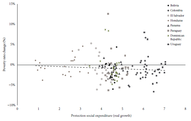
Figure 1 and Figure 2 show the relationship between economic growth and poverty reduction; and social protection spending and poverty reduction respectively, using data from eight Latin American countries from period 2000 to 2019. Although both figures evidence a negative relationship between our variables of analysis, is not possible to conclude if this negative relationship is statistically significant by only looking at the plot; hence, the aim of this paper is to determine and quantify the impact that economic growth and social protection expenditure has had on poverty reduction in Latin American countries for the period 2000-2019. To do so, a Panel is used since it works with cross-section and times series data, simultaneously. Also, the presence of endogeneity in our variables is taken into consideration by the estimation of a Vector Autoregressive (VAR) model. Hence, the paper estimates a Panel Vector Autoregressive (PVAR) model.
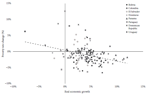
Source: Author’s elaboration based on Economic Commission for Latin America and the Caribbean (ECLAC) data.
Figure 1 Relationship between economic growth and poverty rate in Latin America, 2000-2019
2. LITERATURE REVIEW
2.1. Theoretical framework
Theoretically, there are two approaches in how economic growth could impact on poverty reduction and economic inequalities. The first one is the absolute approach promoted by the World Bank, based on Ravallion and Chen (2001) and Kraay (2004) works in which they point out that economic growth is the most important thing to encourage poverty reduction and the fall of inequality is inherent to it. On the other hand, the relative approach promoted by the works of Kakwani and Son (1990) and Kakwani and Pernia (2000), focuses its objectives on postulating a growth model that, in addition to increasing the income of the poor proportionally more than that of the non-poor, generates long-term distributive changes that manifest themselves in sustained reductions in the levels of inequality.
Hence, the absolute approach ensures that there will be a trickle-down effect due to economic growth that would impact on poverty reduction. This effect is based on Kuznets’s (1955) hypothesis of U inverted shaped economic development, whereas poverty and inequalities will reduce as the economy grows. Nevertheless, Chenery et al. (1974) critiques the trickle-down effect of the economic growth on grounds that it matters, but also public policies focused on pro-distribution in favor to the poorest members of society. Later on, the relative approach based on the pro-distribution concept, sets up the growth pro-poor concept to refer to the economic growth accompanied by public policies that mitigate income inequalities and facilitate employment generation for the poorest.
Both approaches seem to agree on the role of economic growth in poverty reduction; however, the difference between them stems in the role that public policy could have in poverty reduction. While the absolute approach focuses on economic growth; the relative approach also takes into consideration the role of public policy intervention.
2.2. Empirical evidence review
There is few empirical evidence using panel data of how economic growth and public expenditure could reduce poverty rates in Latin America and the Caribbean (LAC) countries; and its results are still not conclusive in terms of the effectiveness of public policies. Some authors argued that public policies focused matters on poverty reduction, some others argued otherwise. However, it is more likely to find evidence in a cross-section data, and its results are conclusive: Economic growth is the principal variable that explains poverty reduction.
Gasparini, Gutierrez, and Tornarolli (2005) were the pioneers to get empirical evidence on how growth impacts on poverty reduction in lac countries from 1989 to 2004. They used microdata from household surveys of 18 LAC countries to evidence that economies have experienced heterogenous patterns of pro-poor economic growth and poverty changes. For instance, there are seven countries which have experienced significant episodes of pro-poor income growth, and nine which have not; therefore, episodes of significant pro-poor income growth over this period have been rare in LAC. On average, economies that have grown (in terms of Gross Domestic Produtc, GDP, per capita) at more than 1% annually have been able to reduce poverty.
However, Azevedo, Inchaust, and Sanfelice (2013) extended the sample until 2010 and used a PVAR model and its variance decomposition of poverty reduction and they concluded that for LAC countries, 34% of poverty reduction is attributable to public policies, in comparison with 66% which is attributable to per capita economic growth. In the same way, Ferreira et al. (2013), the ECLAC (2015), Crespo, Klasen, and Wacker (2016), and Breunig and Majeed (2020) found out that economic growth is the most important variable to explain poverty reduction; followed by public policies intervention. A common feature among these three papers is that they used Panel data estimation to get their results.
It is more likely to find empirical evidence when cross-section data is used. For example, Henoch and Ramón (2015) used the Datt-Ravallion methodology to decompose changes of poverty rate in three components: The role of economic growth, the role of redistributed public policy and an error term. They use data from Chile for the period from 1990 to 2013, and they concluded that economic growth is the principal variable which explains around 67% of the poverty reduction; and although the role of distributed public policies has helped out on poverty reduction, it was not significant.
In the same way, it is possible to find evidence from every LAC country. For instance, in 2012 the director of the Konrad Adenauer Foundation, Olaf Jacob, financed the Regional Program of Social Policies in Latin America to find evidence about the role of social public policies and economic growth in 13 Latin American countries. The studied countries were Argentina, Bolivia, Brazil, Chile, Colombia, Costa Rica, Ecuador, Guatemala, Mexico, Paraguay, Peru, Uruguay and Venezuela. Although each country has its own characteristics, a common feature among them all is that economic growth has played the most important role on poverty reduction, followed by social public policies.
The role of social protection expenditure on poverty reduction, in both short and long run, is supported by the evidence found by Abramo, Cecchini, and Morales (2019) in which the Conditional Cash Transfer (CCT) programs helped with two simultaneous objectives: 1) reduce poverty in the short run by consumption via monetary transfers, and 2) reduce poverty in the long run by human capital formation via conditionalities. They affirm that the effect of the CCT in poverty reduction is greater in the long-term rather than in the short-term.
3. METHODOLOGY
3.1. Variables and data
The sample used in this paper consists of an annually frequency panel dataset of 8 Latin American countries which are: Bolivia, Colombia, Dominican Republic, El Salvador, Honduras, Panama, Paraguay and Uruguay over 2000-2019. The panel data estimated is considered as a macro panel given that the number of periods (20) is greater than the number of units (8), and it is a strongly balanced panel given that there are not missing values1. In total, the panel contains 160 observations and the data was obtained from the statistics released by the ECLAC.
A controversy arises when it comes to work with Latin American data. First, we only work with 8 Latin American countries. Adding more economies to the analysis, will make the model lose some time variables since not all countries start measuring their poverty rate since 2000. Working with more cross-sectional data and fewer times periods have disadvantages of capturing endogeneity in our variables, whereby our results will be biased. On the other hand, not considering important economies in the region such as Brazil or Chile make us lose representativeness in Latin America. We have decided to work with the largest amount of temporal data, thus sacrificing cross-sectional units in order to have unbiased results across the paper.
As we mentioned, the aim of this paper is to determine and quantify the impact that economic growth and social protection expenditure has had on poverty reduction in Latin American countries for the period of 2000-2019. The presence of endogeneity in our variables is corrected by the estimation of a PVAR model. Not considering endogeneity would have made our results to be biased; that is why a PVAR is used. One advantage of estimating a PVAR model is that it estimates the variance decomposition which it allows to quantify the impact of how one shock affects another variable.
The paper uses 3 endogenous variables: The logarithm of the real GDP (constant price of 2010), the percentage of the population living in poverty (measure as a monetary poverty rate) and the logarithm of the central government expenditure in social protection, which could be defined as the range of public policies and social programs needed to reduce the lifelong consequences of poverty exclusion (UNICEF, sf). The paper also considers one exogenous variable, which is a dummy variable that stands for 1 for the global crisis of 2008 and 0 otherwise.
3.2. Analysis procedure
When it comes to working with times series data, we must ensure that all our variable are stationary, otherwise, estimation results are going to be spurious. In order to check the stationarity properties of the variables, the paper uses the Levin, Lin and Chu (LLC) unit root test given that this test is appropriate when the panel cross-section units (8) divided by the size of the panel temporal dimension (20) tends to zero.
Then, if all endogenous variables are integrated of order one (I∼1), a test to determine cointegration must be done. If there is a long-term relationship, a Panel Vector Error Correction (VEC) will be estimated, otherwise it would be a PVAR model. To estimate the optimal lag in our model (see Appendix 1), we use the Akaike Information Criteria (AIC), the Schwarz Criteria (SC) and the Hannan-Quinn Criteria (HQ). All lag length criteria suggest to use 1 optimal lag in our model. The Cholesky’s decomposition was used to estimate our model, where variables are treated from the least to the most endogenous. The logarithm of the GDP (lGDP) is treated as the least endogenous, followed by the central government expenditure on social protection (lSPE) and the most endogenous being the poverty rate (POV). The stability of the PVAR is shown in Appendix 2, where no root lies outside the unit circle, so the specification of our model satisfies the stability condition. We also present, in Appendix 3, that the residuals of the models do not have any serial correlation problem.
After the estimation results, we can draw the impulse response functions (IRFS) to show the response of a particular variable to one standard deviation shock on each and every other variable in the system. In addition, we can display the variance decomposition (VD) in a table to show the proportion of the forecast error variance for each variable that is attributable to its own shocks and shocks in other variables in the system. Finally, a Granger causality test is used to determine whether changes in one variable cause changes in another variable.
3.3. Econometric methodology
The interdependence of relationship between variables could be solved by using a general equilibrium model. These models are useful to provide answers to economic policy issues, however, they impose certain constraints that are not always compatible with the statistical properties of the data (Muinelo-Gallo, Miranda, and Mordecki, 2020). Another way used to solve interdependence, is achieved by constructing a VAR model, where all variables are treated as endogenous variables.
As it was mentioned before, the paper takes into consideration eight units of cross-section analysis and 20 years for each unit, so the paper performs a dynamic empirical analysis of simultaneous equation model using the PVAR methodology. According to Grossmann, Love, and Orlov (2014) a PVAR methodology allows to specify the model with few theoretical information about the relationships among variables. Also, the PVAR methodology is useful when there exists a problem of endogeneity, and, finally, the use of time series and cross section dimension allows us to make more complete use of information.
The paper estimates a PVAR model with three endogenous variables with one optimal lag. Formally:
Where the cross section of the panel is represented by i = 1,2,…,8 and it stands for each country. The time series is represented by t = 1,2,…,20 and it goes from 2000 to 2019. Y it represents the endogenous variables which are a 1×3 vector. The Y it vector of endogenous variables is represented by the GDP (constant price of 2010), the population living in poverty (as a percentage of total population) and the central government expenditure in social protection. Likewise, X it represents the exogenous variable which is a dummy variable that stands for 1 for the global crisis of 2008 and 0 otherwise; while μ i represents the country effects variable that captures the unobservable heterogeneity. Finally, εi is the error term of the model estimated, where is assumed that E(ε it ) = 0, E(ε it ,ε is ) = 0 ∀ t > s.
4. EMPIRICAL RESULTS
In this section, first, we conducted a unit root test to avoid misleading results that are caused by using non-stationary time series data. Second, the estimation result of the PVAR is presented. Then, the impulse response function, variance decomposition and the Granger causality test outcomes will be presented.
4.1. Unit root test
Table 1 presents the main results of the unit root test for the lGDP, the lSPE and the POV. It is found that, both lGDP and lSPE are not stationary in levels, but they are in their first difference, I(1); while POV variable is in its level, I(0).
Table 1 Levin, Lin and Chu unit root test outcomes
| lGDP ∼ I(1) | lSPE ∼ I(1) | POV ∼ I(0) | ||
| LLC test in levels | t-statistic* | 1.6921 | 1.5792 | 3.0881 |
| p-value | 0.9547 | 0.0571 | 0.0010 | |
| Conclusion | Do not reject H0 → Not stationary in levels |
Do not reject H0 → Not stationary in levels |
Reject H0 → Stationary in levels |
|
| LLC test in first difference | t-statistic* | 3.9397 | 11.6477 | - |
| p-value | 0.0000 | 0.0000 | - | |
| Conclusion | Reject H0 → Stationary in first difference |
Reject H0 → Stationary in first difference |
- |
Source: Author’s estimation.
Cointegration exists when these two requirements are met: All variables are integrated in the same order, normally speaking it is said that variables are integrated of order one, I(1); and the error term of the model is stationary at its level, I(0). Before performing a cointegration test we must ensure that these requirements are met. In Table 1, we can see that not all variables are integrated in the same order, so the requirements to perform a cointegration test has not been met, so we proceed to estimate a PVAR.
4.2. Estimation result
Estimating a PVAR model implies that all variables are treated as endogenous, that is to say that each variable is affected by the others; however, Cholesky’s decomposition works to set up an order from the least endogenous variable to the most. According to the literature review section, Cholesky’s decomposition is as follow: The lGDP will impact on the lSPE and this will on the POV.
Table 2 presents the main results of our PVAR estimation. As we can see, all endogenous variables are statistically significant to explain the POV variable, being the most important the first lag of the lGDP and the lag of the POV, both of them at 99% level of confidence; followed by the lSPE at 90% level of confidence. These results are according with the empirical evidence previous mentioned, where the economic growth is the most important variable followed by public policy spending to explain poverty reduction.
Table 2 PVAR estimation output
| D(lGDP) | D(lSPE) | POV | |
| First lag of D(lGDP) | 0.2864 *** (0.079) |
0.3100 (0.218) |
-10.547 *** (2.312) |
| First lag of D(lSPE) | 0.0203 (0.026) |
-0.0350 (0.072) |
-1.3089 * (0.765) |
| First lag of POV | -0.0011 ** (0.000) |
0.0001 (0.001) |
0.9944 *** (0.016) |
| Constant | 0.0004 (0.000) |
0.0143 (0.067) |
0.0623 (0.710) |
| DUM1 | 0.0798 *** (0.035) |
0.1110 (0.0672) |
1.144 (1.039) |
Note: Standard errors in ( ). *** 99% significance, ** 95% significance, * 90% significance.
Source: Author’s estimation.
4.3. Post estimation test
An important utility to use a PVAR estimation is that it allows the dynamic analysis of the series. In this subsection, first we report the impulse response function, then the variance decomposition and, finally, the Granger causality test outcome is presented.
4.3.1. Impulse response function (IRF)
According to Hamilton (1994) and Enders (2015), the impulse response function (IRF) works to describe the effect of an innovation in the jth variable on future values of each of the variable in the system. In other words, the aim of the IRF is to describe how a shock in certain variable would impact on the present and future of another variable. Figure 3 graphs the POV orthogonal response due to impulse or shock from lGDP and lSPE, in one standard deviation magnitude. The solid lines represent the impulse responses, and the dashed lines represent a 95% confidence interval.

As we can see from Figure 3, one standard deviation shock on the change of the lGDP causes a significant decrease in the poverty rate for twenty periods after which the effect dissipates. However, one standard deviation shock to the change of the logarithm of social protection expenditure does not show any significant movement in the poverty rate.
4.3.2. Variance decomposition (VD)
The variance decomposition (VD) is the proportion of the forecast error variance that is attributable to its own shocks and shocks in other variables in the system. From Table 3, we can conclude that POV variable explains the preponderance of its own past values at short forecast horizons, but after a time, the change in lGDP gains preponderance to explains the change in the poverty rate.
Table 3 Variance decomposition of POV
| Step | ∆lGDP | ∆lSPE | ∆POV | Step | ∆lGDP | ∆lSPE | ∆POV |
| 1 | 9.705 | 0.050 | 90.244 | 11 | 40.141 | 5.781 | 54.076 |
| 2 | 22.042 | 0.210 | 77.747 | 12 | 40.287 | 6.795 | 52.916 |
| 3 | 29.172 | 0.512 | 65.684 | 13 | 40.334 | 7.829 | 51.835 |
| 4 | 33.360 | 0.953 | 65.866 | 14 | 40.305 | 8.874 | 50.820 |
| 5 | 35.944 | 1.525 | 62.530 | 15 | 40.219 | 9.9195 | 49.860 |
| 6 | 37.601 | 2.214 | 60.184 | 16 | 40.090 | 10.957 | 48.952 |
| 7 | 38.688 | 3.001 | 58.310 | 17 | 39.927 | 11.981 | 48.091 |
| 8 | 39.403 | 3.869 | 56.727 | 18 | 39.741 | 12.985 | 47.273 |
| 9 | 39.863 | 4.801 | 55.335 | 19 | 39.537 | 13.966 | 46.496 |
| 10 | 40.141 | 5.782 | 54.076 | 20 | 39.096 | 15.847 | 45.056 |
Source: Author’s estimation.
Table 3 presents the accumulated response of POV variable to one standard deviation shock of lGDP and lSPE. The accumulated effect after 20 periods is that when there is an increment of one standard deviation shock of lGDP, the poverty rate will change by 39.09; while when there is an increment of one standard deviation shock of lSPE, the poverty rate will change only by 15.84. It is also possible to obtain the elasticities knowing the standard deviation of each variable. The standard deviation of lGDP is 0.964902, while for lSPE is 1.3266; therefore, the cumulative effect of a change in lGDP and in lSPE of one percentage point affects the poverty rate change by 37.72 and 21.02, respectively.
4.3.3. Granger causality
In order to observe if causality exits between variables, the Granger causality test is carried out (Granger, 1969). This test does not imply causality, but it points out that a variable causes changes in another variable if both past and present values of the former variable help to predict the latter variable. Wooldridge (2010) and Gujarati and Porter (2009) explain that the Granger causality test assumes that the relevant information to the prediction is contained solely in the time series data of the variables.
The results shown in Table 4 are as we expected, and they reaffirm our Cholesky’s decomposition of the variables. We can conclude that there is a bidirectional Granger causality process between lGDP and POV because both Granger causes each other. On the other hand, the lSPE variable does not Granger cause POV at 5% level of significance, however, it does at 10%.
Table 4 Granger causality test
| → Granger causality | p-value | Conclusion (5% level of significance) |
| D(lGDP) → D(lSPE) | 0.1041 | No Granger causality |
| D(lGDP) → POV | 0.0000 | Granger Causality |
| D(lSPE) → POV | 0.0590 | No Granger causality |
| POV → D(lGDP) | 0.0498 | Granger Causality |
| D(lSPE) → D(lGDP) | 0.4358 | No Granger causality |
| POV → D(lSPE) | 0.9385 | No Granger Causality |
Source: Author’s estimation.
4.4. Cross-section analysis
The results show that economic growth has the strongest influence on poverty reduction, in both short and long run, however, there is heterogeneity of economic growth in poverty reduction as evidenced in each country. For instance, in absolute values, Bolivia was the country that has experienced the greatest reduction in its poverty rate, going from 66.4% in 2000 to 43.6% in 2019.Nevertheless, in relative values, El Salvador was the country which has a better performance in reducing its poverty rate in terms of economic growth: Its elasticity was of -4.1%, it means that a 1% economic growth is associated with a poverty reduction of 4.1%, followed by Colombia (-2.9%) and Bolivia (-2.8%) [See Table 5].
Table 5 Elasticity economic growth and poverty reduction, 2000-2019
| Country | Poverty rate reduction |
Economic growth (yearly mean) |
Elasticity |
| El Salvador | -12.6 | 3.826 | -3.3 |
| Colombia | -17.4 | 6.038 | -2.9 |
| Bolivia | -22.8 | 8.005 | -2.8 |
| Uruguay | -11.4 | 5.201 | -2.2 |
| Paraguay | -17.8 | 8.235 | -2.2 |
| Dominican Republic | -8.4 | 6.534 | -1.3 |
| Panama | -5.8 | 7.821 | -0.7 |
| Honduras | 5.0 | 6.266 | 0.8 |
Source: Author’s estimation.
The only country which has experienced an increase in its poverty rate during the same period of analysis was Honduras and this is because its private investment is limited by low economic returns to investment due to 1) inadequate education of its labor force, 2) high administrative costs and 3) crime and security (U.S. Agency for International Development, 2021).
5. CONCLUDING REMARKS AND POLICY RECOMENDATION
The results show that economic growth has the strongest influence, in both short and long run, on poverty reduction; while the impact of social protection expenditure does not seem to be significant in short forecast horizons, it seems to be in the long run. According to our forecast error variance decomposition, at period 20, around 40% of poverty reduction is explained by a change in the economic growth; while almost 16% is explained by a change in the social protection expenditure.
The evidence presented in this paper is supported from a theoretical and empirical approach. From the theoretical approach, the absolute and relative approach proposed the importance of economic growth on poverty reduction as the most important variable. The relative approach, points out that it is also important to consider policy intervention. From empirical evidence, and using grouped data, similar results were found on works from Azevedo, Inchaust, and Sanfelice (2013) where they found that 34% of poverty reduction is attributable to public policies, in comparison with 66% which is attributable to per capita economic growth. Likewise, Ferreira et al. (2013); Crespo, Klasen, and Wacker (2016) and Breunig and Majeed (2020) found similar results. Furthermore, using cross-section data, Jacob (2012) found in 13 LAC that economic growth has played the most important role in poverty reduction, followed by social public policies. Same results were obtained by Henoch and Ramón (2015), for Chile, where economic growth has been the principal variable which explains around 67% of the poverty reduction; and although the role of distributed public policies has helped out in poverty reduction, it was not significant.
Although public policies have a lesser impact on poverty reduction in the short run, as time passes by, the impact of policy intervention becomes more important to explain changes in poverty rates. This is supported by the evidence shown by Jacob (2012) and Abramo, Cecchini, and Morales (2019). Therefore, as Harberger (1990) said, the role of public policies is not to give heaven to everyone, but to get out of hell to those who are there.
6. LIMITATIONS
Limitations come from the data. First, missing values cause to face trade-off between choosing more cross-section units and less time series, or vice versa. It decides to choose the number of units in which the temporal series have the largest amount of available data in common. In other words, we have decided to sacrifice some cross-sections units for time series data. If more units would have been chosen instead of time series data, a PVAR estimation would have been biased and inefficient due to the lower amount of time series data (Baltagi, 2021). Definitely, in the future, further research would not face this trade off, because it will be possible to take into consideration more time series data and cross-section units together. If it is so, results will be more robust.
Moreover, some missing values are filled out with data released by their respective National Statistic Institutions. However, in the particular case of the Colombian economy, the Kalman smoothing interpolation is used to complete the data of the poverty rate for the years 2006 and 2007; and this is why The Colombian National Statistical System (DANE) does not report the poverty rate for these years due to the change of the methodology.
Finally, for further investigation, robustness results could be found if CCT on social programs data is used in comparison with social protection expenditure. However, the principal limitation now is the lack of CCT database.


