


 nova página do texto(beta)
 Inglês (pdf)
 Artigo em XML
 Referências do artigo
 Enviar este artigo por email
 Citado por SciELO
  Similares em
SciELO
Similares em
SciELO 
 Permalink
1. Introduction
In the last decades, US Economic Policy Uncertainty (USEPU) has been related to the irregular federal immigration policy, the constant risk of prolonged government shutdowns, the quantitative easing (QE) programs and, of course, the subprime mortgages crisis and its short- and long-run side effects. These uncertainty sources have had special impact on economic and financial variables in global markets, and particularly in the emerging ones. More recently, the USEPU has received special attention due in part to the fiscal situation of US government, the uncertain monetary policy, the prevailing consequences of the trade war between US and China, the doubtful energy policy, the need of an integral strategy adjacent to the COVID-19 pandemic, and the course of policy to be followed by the new administration of the federal government. All those events may cause uncertainty outside of US in the behavior of financial markets, and in particular in stock markets (Balli et al., 2017).
Research on evaluating the impact of the USEPU on global stock markets has been on the rise in recent years. For instance, Li et al. (2020) use a continuous and discrete wavelet approach to assess the dynamic correlation and causality between the USEPU and the stock markets in India and China in the period 1997-2018. The authors use Granger causality tests and find that the relationship between USEPU and stock returns in both countries is weak in the short run but gradually becomes stronger in the long run. Likewise, Zhang et al. (2019) find that the trade war between US and China caused substantial uncertainty in stock markets. The authors ascertain that, although China has become more influential, US dominant position still holds in these markets. Their results suggest that concerns are more likely to be driven by political factors rather than economic ones. On the other hand, Antonakakis et al. (2017) examine whether stock returns in US and their volatility can be predicted through economic uncertainty indicators by means of a nonparametric causality-in-quantile approach. Their findings reveal that USEPU possess predictive information for US stock returns and volatility, barring few cases. More generally, Balcilar et al. (2019) examine whether stock returns and volatility in Hong Kong, Malaysia and South Korea can be predicted by using the EPU indexes of US, China, Euro Zone, and Japan. In their study, linear Granger causality tests fail to find evidence of predictability, barring the case of South Korean EPU predicting its own stock returns. Moreover, the authors use a nonparametric causality-in-quantiles test detecting strong evidence of causality from the EPUs towards stock return volatility in Malaysia and toward returns and volatility in South Korea. There is no evidence of predictability from EPUs for return and volatility of the Hong Kong stock market.
More generally, recent investigations state that for emerging stock markets, the USEPU is related to stock market declines (Mishra and Debata, 2020), which might be attributed to the incentives and competition of risk managers to hide negative news that lessen the impact of high levels in the USEPU (Luo and Zhang, 2020) and veil the existence of asymmetric, nonlinear, and non-monotonous relationships in the stock markets in an uncertain environment (Hoque and Zaidi, 2019). Finally, the specialized literature shows that there are low-frequency cycles between the USEPU and stock markets (Ko and Lee, 2015).
The impact of the USEPU on different economic and financial variables for Latin American countries has been studied by Alam and Istiak (2020) for the Mexican interest rate, Cerda, Silva, and Valente (2018) for the Chilean fall in Gross Domestic Product (GDP), investment, and employment during the last 23 years, Choi and Shim (2019) for volatility in macroeconomic variables in Brazil and Chile, and Coronado, Martínez, and Venegas-Martínez (2020) for macroeconomic variables (exchange rate, consumer price index, industrial production, and interest rates) of major Latin American Countries. Finally, Gil-León and Silva-Pinzón (2019) study the impact of Colombia’s economic policy uncertainty on investors through a var analysis, and find a negative investors’ response.
Needless to say, there is a lack in the literature of an up-to-date, long-term and time-varying analysis of the indirect effects of the USEPU on the main stock markets in Latin America. The main objective of this investigation is to inquire about the relationship between the evolution of the USEPU index and the dynamic behavior of a sample of the stock markets of the major Latin American Countries: Colombia, Chile, Brazil, and Mexico. To do this, a Time-Varying Bayesian Structural Vector Autoregressive (TVB-SVAR) model and a Time-Varying Granger-causality (TV-GC) test are applied.
This research is distinguished from other studies on the subject in the following aspects: 1) it uses a TVB-SVAR; 2) it uses a tv-gc test; 3) it carries out a Residual Augmented Least Squares (RALS) test for unit roots that improves the power when the error term follows a non-normal distribution; 4) it uses the longest period compared with other studies and is updated to 2020 including the COVID-19 pandemic; and 5) it compares the magnitude of USEPU’s impact across markets.
The present research is organized as follows: Section 2 describes the methodology to be used in this research; section 3 depicts database sources, section 4 provides the descriptive statistics of the variables under study and carries out a test for unit roots; section 5 states the time-varying Bayesian econometric methodology; section 6 provides the results from the Time-Varying Impulse-Response Functions (TV-IRFS); section 7 presents the main results of the time-varying Granger-causality test; and section 8 concludes, provides policy recommendations and acknowledges limitations.
2. Methodology
In order to have a satisfactory measure of USEPU, this research uses an index prepared, monthly, by an international agency “Economic Policy Uncertainty” dedicated to calculating this measure for many countries since 1985. This index is computed in accordance to the methodology proposed by Baker et al. (2016).
The USEPU considers three main aspects. The first one quantifies the news coverage of policy-related economic uncertainty. The second one contains the federal tax code provisions that will expire in future years. The last one uses disagreement among economic forecasters as a proxy for uncertainty.
More specifically, the first aspect considers the volume of news articles that talk about the uncertainty of US economic policy in the main newspapers: USA Today, The Miami Herald, The Chicago Tribune, The Washington Post, The Los Angeles Times, The Boston Globe, The San Francisco Chronicle, The Dallas Morning News, The Houston Chronicle, and The Wall Street Journal.
The second aspect of the index is based on reports from the Congressional Budget Office (CBO) that compiles a list of temporary provisions of the federal tax code. In order to do that, annual dollar-weighted numbers of tax code provisions scheduled to expire over the next 10 years are considered. This provides a measure of the level of uncertainty of the path the federal tax code will take in the future.
The third aspect of the policy-related uncertainty index is based on a survey of professional forecasters of the Federal Reserve Bank of Philadelphia (FED-P). In this case, the dispersion between individual forecasters’ predictions of future levels of the consumer price index, federal expenditures, and state and local expenditures are used to construct indices of uncertainty about policy-related macroeconomic variables.
Subsequently, the relationship between the USEPU and the returns of the stock markets of the sample of Latin American countries is examined through a TVB-SVAR model by using the Bayesian Estimation, Analysis and Regression (BEAR) toolbox for forecasting and policy analysis, which is a MATLAB-based toolbox developed by The European Central Bank and available for free use1.
3. Data sources
This research considers a sample of four of the major Latin American Countries (LAC): Chile, Brazil, Mexico and Colombia. Hence, the database consists of four series of stock market indexes: Chile’s IPSA (Índice de Precios Selectivo de Acciones) index, Brazil’s IBOV (abbreviated name of IBOVESPA, Índice da Bolsa de Valores de São Paulo) index, Mexico’s MEXBOL (Mexican Bolsa) index and Colombia’s COLCAP (Colombia Capital) index, all of them obtained from Bloomberg for the period 08/01/2002-8/1/2020, which gives a total of 217 monthly observations for each index. On the other hand, the USEPU is obtained from the website of Economic Policy Uncertainty Index (EPUI) and generated in accordance to the methodology proposed by Baker et al. (2016) 2. The five series are transformed into logarithmic growth rates, or logarithmic returns, given by (In (p t ) - In (p t-1 )) × 100. Figure 1 shows all series as growth rates.
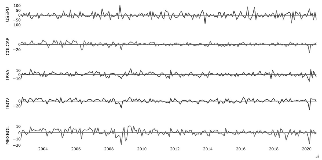
Source: Authors’ own elaboration from Bloomberg Database and USEPU processed with Gauss.
Figure 1 Logarithmic growth rates of USEPU, COLCAP, IPSA, IBOV and MEXBOL, 08/01/2002 to 8/1/2020
Note that the logarithmic growth rates have similar dynamics at various times, and there is a significant break in the USEPU series (USEPU growth rates) in late 2008 and early 2009, which coincides with the subprime mortgage crisis that affected the stock markets of the economies considered in the sample; and, of course, many others. There is also a significant drop in the USEPU at the beginning of the second half of 2011, which coincides with the European debt crisis in August 2011. The same occurred in 2012 and 2013, which could be attributed to US fiscal crisis and the government shutdowns in these years. Another peak in the USEPU growth rates occurred in early 2017, which agrees with the election victory of US President Trump. For 2020, all series decrease over the year, which could reflect the partial impacts of the COVID-19 pandemic in the world.
4. Descriptive statistics and unit roots
Descriptive statistics of all series are presented in Table 1. The statistics show that the series do not follow a normal distribution according to normality test of Jarque and Bera (1980). This can be explained in part by the excess kurtosis and positive asymmetry for the USEPU, as well as negative asymmetry for the rest of the series. Table 2 presents the RALS unit-root tests results3, which has the advantage of been applied to time series that are not normally distributed (Coronado et al. 2018). In fact, RALS test improves power when the error term follows a non-normal distribution. For instance, the RALS test is more powerful than the Dickey-Fuller test which does not incorporate information on non-normal errors.
Table 1 Summary of descriptive statistics
| Variable | USEPU | COLCAP | IPSA | IBOV | MEXBOL |
|---|---|---|---|---|---|
| Mean | 0.306 | 1.015 | 0.604 | 1.046 | 0.824 |
| Median | -1.504 | 1.158 | 0.450 | 0.942 | 0.943 |
| Min | -91.889 | -32.124 | -16.731 | -35.531 | -19.667 |
| Max | 107.653 | 16.389 | 14.916 | 16.484 | 10.954 |
| Var | 813.135 | 39.523 | 22.261 | 49.177 | 4.729 |
| Sd | 28.516 | 6.287 | 4.718 | 7.013 | 4.729 |
| Skew | 0.312 | -0.841 | -0.076 | -1.001 | -0.835 |
| Kurt | 4.130 | 7.192 | 3.767 | 6.697 | 5.072 |
| Jarque-Bera | 15.005* | 183.610* | 5.505** | 159.060* | 63.755* |
Notes: * Values are significant at the 1% level, and ** values are significant at the 5% level.
Source: Authors’ own elaboration from Bloomberg Database and USEPU with STATA.
5. Setting the bayesian methodology
To examine the behavior between the USEPU and the rest of the series, a TVB-SVAR model is applied. This model differs from a model of fixed coefficients in that the model parameters vary over time according to the underlying laws of motion (Del Negro, 2012; Lubik and Matthes, 2016; Miranda-Agrippino and Ricco, 2018).
The model specification is defined through a vector of endogenous variables y = [USEPU, COLCOP, IPSA, MEXBOL]. All series are specified as logarithmic growth rates. The lag(3) was chosen based on the Schwarz-Bayesian criteria (Schwarz, 1978). The model was estimated using the BEAR toolbox4, specifically using Bayesian techniques and disperse matrices (Dieppe, Legrand, and Van Roye, 2016 and 2018; Legrand, 2019; Pham and Sala, 2019; Zlobins, 2019). Specifically, the model is expressed as:
where A i,t , i = 1,2,…,p, are the matrices of parameters that vary over time. This model could be specified in its compact form as:
where
The VAR coefficients are assumed to follow the autoregressive process:
Next, the covariance matrix Ʃt in
where
where
6. Time-varying impulse-renponse functions (IRFS)
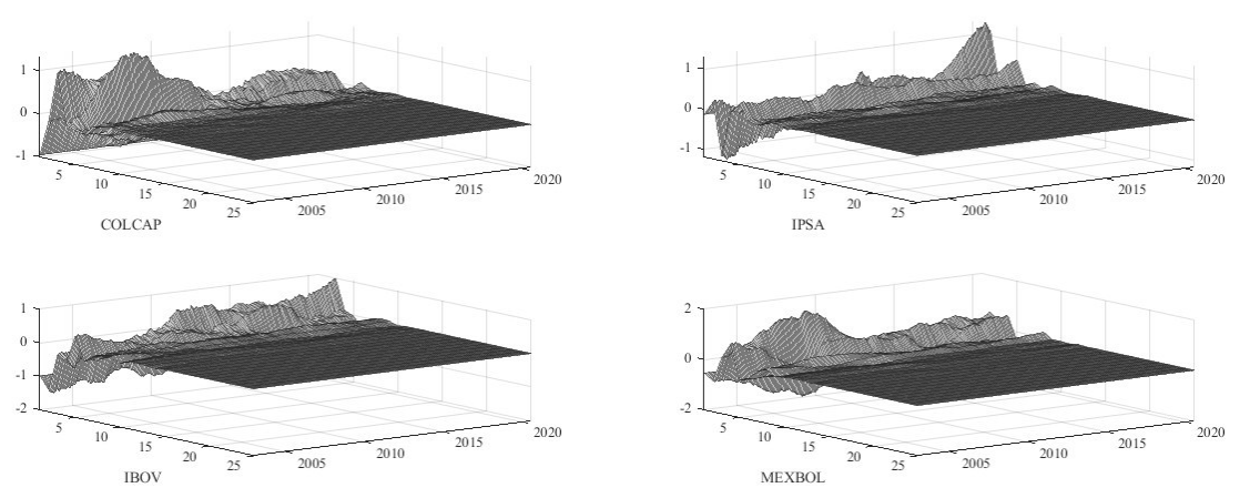
This section presents the results from the IRFs and surfaces of irfs over time. Figure 2 shows the IRFs results of a shock from the USEPU to the four stock market returns of the LAC under study. A USEPU shock initially affects the stock market returns in a negative manner and, subsequently, the effect becomes positive reaching its maximum level around the third period (three months) for the cases of the IPSA, IBOV and MEXBOL. The same is true for the COLCAP but on a smaller scale. The effects of the USEPU shock dissipates completely around period twenty for COLCAP, IPSA, and IBOV, and around period twenty-three for the Mexican stock market (almost two years in all cases). These results show the impacts of USEPU and how they are transmitted over time to stock markets in lac. Moreover, Figure 3 shows the IRFs over time, or time-varying IRFs, of a shock from USEPU: On the axis of the horizontal plane in Figure 3 the years 2005, 2010, 2015 and 2020 are shown; the irfs are shown over time. It is observed, as time passes, that the effect of the shock is similar in all the indices, although the magnitude of the shocks for IPSA and IBOV are greater in the initial periods of 2002-2010 while for COLCAP and MEXBOL are greater in the initial periods of 2011-2020. Finally, the scale for the COLCAP is lower compared with the other three indexes. The results show how a USEPU shock to lac stock market returns first appears and then turns positive with different magnitudes and durations. This could have been considered by economic agents as an investment diversification strategy for the period prior to COVID-19 (Christou et al., 2017).
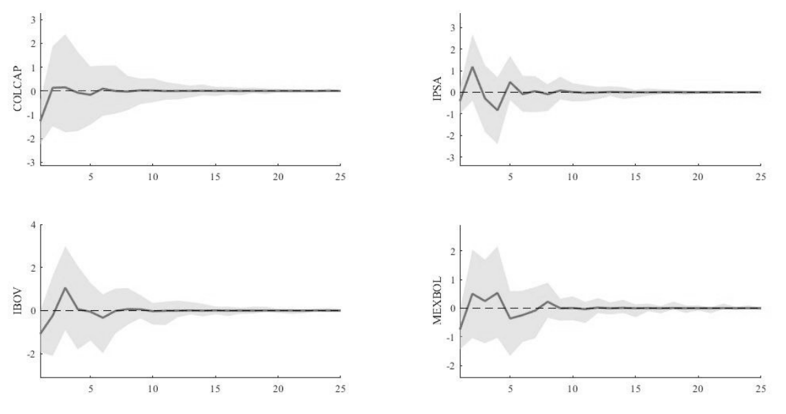
Source: Authors’ own elaboration from Bloomberg Database and USEPU with BEAR toolbox.
Figure 2 Impulse-response functions from a shock from the USEPU to COLCAP, IPSA, IBOV, and MEXBOL returns
7. Time-varying granger-causality test
In order to corroborate the impact from the USEPU index on the four stock market
returns, a Time-Varying Granger-Causality test is applied6. The TVB-SVAR model for a time series described as
where εt,T is a mean zero vector of independent random perturbancs, u(t/T) is a vector of intercepts, and Al (t/T), l = 1,2,…,p, are the autoregressive coefficient matrices. Each VAR coefficient is described as a function of time. In this case, the B-spline expansion can be used to represent this function. Subsequently, each intercept and autoregressive time function is a linear combination of the B-spline functions as:
where Ψk (t) are the B-spline functions
(Ψ0 = 1 = constant for all t),
M is the number of functions used in the B-spline expansion,
and
where u
k
are vectors and
The TV-GC test can be carried out by testing whether or not there is at least one autoregressive time function from y jt to y lt different from at least at one point in time. In other words, the TV-GC tests whether or not at least one coefficient from the B-spline expansion of the autoregressive time functions is different from zero.
The model parametrization allows us to test whether the Granger causality between two time series varies over time or not. In this case, the null hypothesis is H0 = is constant over time and the alternative hypothesis is H1 = it varies over time7.
Table 3 shows the results from the TV-GC test. All results are statistically significant, which implies that the USEPU Granger-causes the stock market returns. That is, the USEPU index Granger-causes the stock market returns at least at one point in time. These results corroborate the findings from the irfs presented previously in Figures 3 and 4.
Table 3 Granger causality test results
| Causality hyphotesis | TV-GC test |
|---|---|
| USEPU → COLCAP | 0.062* |
| EPU → IPSA | 0.038** |
| EPU → IBOV | 0.091* |
| EPU → MEXBOL | 0.000*** |
Note: The results are statistically significant at the 1% level (***), 5% level (**), and 10% (*)
Source: Authors’ own elaboration from Bloomberg Database and EPUI with R platform.
It can be noted in Table 3 that the TV-GC test corroborated that the USEPU index Granger- causes the stock market returns at least at one point in time.
8. Conclusions
In order to study the relationship between the USEPU and the chosen sample of stock markets of LAC, a TVB-SVAR model was applied. The IRFs from a USEPU shock to the Colombia’s COLCAP index, Chile’s IPSA index, Brazil’s IBOV index, and Mexico’s MEXBOL index were estimated using the bear toolbox. The results showed that a USEPU shock initially affects the stock market returns negatively and then its effect becomes positive, reaching its maximum level around the third period in the cases of the IPSA, IBOV, and MEXBOL. The same happens with COLCAP but on a smaller scale.
These results demonstrate the impacts of news, reports from CBO and surveys from FED-P in the US and how they are transmitted over time to stock markets in Latin America. Regarding the time-varying irf, as time passes the effect of the shock is similar in all the indices, although the magnitude of the shocks for IPSA and IBOV are higher in the initial periods of 2002-2010 while for COLCAP and MEXBOL are higher in the initial periods of 2011-2020. Finally, in order to corroborate these results, the tv-gc corroborated the findings from the irfs. The results show that the USEPU Granger-causes the Latin American stock market returns at least at one point in time.
This research has a dual purpose: 1) to study the effects of the USEPU on the main Latin American stock exchanges, and 2) to analyze the expected repercussions on the stock exchanges of underdeveloped economies with conditions similar to the sample under study. As a conclusion of this study, the possible consequence, within a broader and longer-term framework that includes the role of the new international conditions in the US, is that the USEPU may delay the investments of companies and investors in the stock markets of similar emerging economies (as a contagion effect), which in turn can retard economic growth. For example, in the first quarter of 2015 the market capitalization value of the Mexican Stock Exchange represented 43.38% of GDP, while in the second quarter of 2020 it represented 37.46%.
Regarding recommendations, and in particular to the oil-producing countries, it is important to compare, first of all, the cases of Mexico and Colombia. In the Mexican case, a USEPU shock negatively affects the stock market, reaching its maximum level around the third period. However, the impact for the Colombian COLCAP is lower. This may be due to the fact that the company that explores, produces and imports oil in Colombia, Ecopetrol, has a mixed participation between the government and local and foreign investors, being a listed company on the Colombian Stock Exchange. On the other hand, with respect to Brazil, Petrobras currently operates in the stock market as a semi-public company, mainly owned by the government, with private participation, and the USEPU shocks also last less than in the Mexican case. In summary, private participation in state oil companies reduces the impact of the USEPU, leading to the recommendation that similar emerging oil-producing economies become semi-public listed on the stock exchange, as the government can influence in the operation of the market to reduce the impact.
It is worth mentioning that the research by Alam and Istiak (2020) for the Mexican case on the effects of a USEPU shock on another relevant financial variable, such as the interest rate, is in line with our conclusions since these authors find that an increase in the USEPU negatively affects the Mexican interest rate.
Finally, a limitation of this study, and potential extension of this work, is that we do not consider the volatilities of the stock market returns to assess whether or not the USEPU has the same impact on Latin American stock markets. To do so, other variables like the VIX volatility index will be considered in the future research agenda to analyze any patterns or trends in a sample of LAC.

