


 nueva página del texto (beta)
 Inglés (pdf)
 Artículo en XML
 Referencias del artículo
 Enviar artículo por email
 Citado por SciELO
  Similares en
SciELO
Similares en
SciELO 
 Permalink
1. Introduction
Mexico suffers of high poverty levels. According to official poverty records, 40% of the population lives in poverty, and in 2018 almost a tenth of the population lived in extreme poverty (Consejo Nacional de Evaluación de la Política de Desarrollo Social, CONEVAL, 2019a). To attend this critical issue, Mexico has pioneered high scale conditional and unconditional programs to support the welfare of the poorest households. Examples of such programs are Oportunidades, formerly Progresa, Adulto Mayor and Procampo. Oportunidades consists of transfers of money conditional to households' human capital investment on the children, while Adulto Mayor consists of non-compensatory pensions and Procampo gives unconditionally transfers to farmers. In 2018, Mexico spent more than seven billion dollars in these social programs.
These program’s micro-effects on health, education and welfare of households have been documented in a series of studies, especially Oportunidades. Behrman, Sengupta and Todd (2005) compared the school outcomes of the children that participated in the program in the first two years of operation with a sample of children not enrolled in Progresa, finding significant benefits in terms of higher school enrollment, lower repetition rates, lower dropout rates and higher re-entry rates in case of dropouts. Regarding the Progresa nutritional supplement, Behrman and Hoddinott (2005) showed a positive effect of the supplement on children between 12 and 36 months of the order of 16% in the mean growth of the children. Barham and Rowberry (2013) found a 4% reduction in the mortality rate associated with diabetes and hypertension in the municipalities where Progresa gained penetration. Finally, Behrman, Parker and Todd (2011) showed that children under the program achieved one more grade of schooling and old youth were more prone to work in the none-agricultural sector.
Macro studies of social programs in Mexico are scarce, two studies have applied linear general equilibrium models to assess the intersectoral and distributional effects of Oportunidades (Beltran, Cardenette and Delgado, 2019) and Aguayo et al. (2009). Both built a social accounting matrix to assess the income generation and income redistribution of an exogenous injection or extraction of resources of the amount that Oportunidades represented. Although they advanced in the macro analysis of the social programs, their results are limited in terms of programs coverage and because of unrealistic theoretical assumptions, among them that all income elasticities of goods and services are one and that induced income distribution effects do not affect poverty measures.
This paper contributes to the line of research of poverty in the context of general equilibrium models. We compare Mexico’s poverty level with the one that would prevail in the case all the three mentioned programs were eliminated at all. This is known as an extraction exercise.
Even though this type of exercise has been done before, especially in Beltran, Cardenette and Delgado (2019), our study expands the analysis in four different ways. First, the sample of programs is larger, as it considers the Adulto Mayor and Procampo programs, in addition to Oportunidades. Second, it abandons the assumption that all goods and services have unitary income elasticities, as we prove that over seventy percent of the sectors have income elasticities different from one. To do this, we estimate the marginal propensities to consume employing a Quadratic Almost Ideal Demand System (QAIDS). In this sense, we construct a fixed price multipliers model which combines, in a simple way, a Social Accounting Matrix (SAM) and micro-data econometric estimations of the consumption block, that represents at least two thirds of the aggregate spending.
Third, we adjust the labor sector’s income by recording salaries received for employers, self-employment, and workers receiving no wages. To this end, shadow wages were estimated employing Mincerian equations (Ayala and Chapa, 2014). As in the case of the income elasticities, the adjustment is not minor: More than half of the workers in Mexico are not incorporated to any social security system, and most of them self-employed. Fourth and finally, contrary to previous studies that assumed inequality remained unchanged when the public transfers are applied, we consider the income distribution effect on poverty. Our findings suggest that Mexico's social programs contribute to alleviate poverty not only for the direct and indirect effect of the money transfers, but also for reducing inequality in the income distribution.
For rest of the paper, section two presents a brief review of the essential features of the three programs considered. Section three describes the various models and estimations we use in the paper, including the SAM model, the qaids estimation of the income elasticities, and the elasticities of the Foster, Greer and Thorbecke (1984) poverty measures to income mean and Gini inequality along the lines of Kakwani (1993) and Huppi and Ravallion (1991). Finally, section four elaborates on the extraction simulation results, offering some concluding remarks.
2. Oportunidades, Adulto mayor and Procampo programs’ features
In 2018, these three programs accounted for almost half of the budget destined to the 67 social programs of the federal government in Mexico, receiving a total budget of 14.3 billion of US dollars. Oportunidades contributed with 28.4%, Adulto Mayor with 13.4% and Procampo with 5.7%.
Oportunidades was initially conceived as a conditional transfer program named Progresa, targeting households in extreme poverty living in rural areas. In 2002 it changed its name for Oportunidades, and in 2014 to Prospera, extending then its coverage to semi-urban and urban areas. In general, the program makes a transfer for each child enrolled in primary or secondary education. The transfer amount ranges between 40 to 60 dollars per month. The household is conditioned to keeping the children in school, as well as making sure they attend scheduled medical consultations and other health services.
When started, the program reached 300,705 households, equivalent to 1.55% of Mexico’s population. As the program changed names it also extended its coverage. In 2008 it covered 5 million households, that is 25 million of inhabitants or 22.2% of the total population. In 2018 it reached 6.5 million of households or 24.1% of the population (CONEVAL, 2019b).
The Adulto Mayor program was created in 2007 targeting adults 70 years old or older living in rural areas, who did not receive any type of pension. That year, the program made transfers to one million of adults or 11.6% of the total target population. In 2008 it attended 1.8 million of beneficiaries, making an unconditional transfer of 45 dollars bi-monthly per-beneficiary. In the following years the program extended its coverage to semi-urban areas and reduced the threshold age to 65 years old. In 2014, it supported 43.8% of the total population of 65 years old or more, transferring 55 dollars bi-monthly to each recipient. In 2019, at the beginning of the Lopez Obrador administration, the program was expanded to all adults of 68 years old (65 years in indigenous villages), regardless of their socioeconomic status or if the beneficiary already received another type of pension or not. Additionally, the transfer was increased substantially, to 132 dollars bi-monthly.
Finally, Procampo is designed to improve the incomes of rural farmers, especially the poorest ones. Launched in 1994, the program established an unconditional annual payment by hectare to the farmers. Starting in 2001, the operating rules considered stratifications in the beneficiaries with the aim of favoring producers with fewer resources, these stratifications had different implications in terms of the monetary amount and the number of hectares supported. In 1994 the program aided 0.542 million beneficiaries, while by 2008 the number of beneficiaries amounted to 2,866 million (Auditoría Superior de la Federación, ASF, 2017).
3. Social accounting matrix multipliers and poverty elasticities: methodology
3.1. A Social Accounting Matrix for Mexico
A SAM is a square matrix in which rows and columns are labeled an “account” or “institutional sector.” Since the SAM reflects where the income comes from (income row) and how it is spent (expenditure column), it must balance perfectly: For each account, the income must be equal to the expenditure. In general, the accounts are divided into economic sectors, factors of production and institutions (e.g., households, the government, the rest of the world). In this way, a SAM identifies the circular flow of income between the agents participating in an economy: Households, primary factors, enterprises or sectors, the government, and foreign transactions.
For our estimations, we use a SAM built in 2008 (Chapa and Ramírez, 2018)1. The SAM was constructed using a “bottom up” method, implying that the Input-Output Table (IOT) is disaggregated by labor and household types using microdata of surveys. For example, the sectorial labor income from the IOT is displayed by gender and occupation using the microdata of the Encuesta Nacional de Ocupación y Empleo 2008 (ENOE 2008) compiled by the Instituto Nacional de Estadística y Geografía (INEGI, 2008). Meanwhile, the income and expenditure by household types are disaggregated using the Encuesta Nacional de Ingresos y Gastos de los Hogares 2008 (ENIGH 2008), also from INEGI (2009). Other sources used are the Cuentas por Sectores Institucionales 2008 (CSI) from INEGI (2014), Secretaría de Hacienda y Crédito Público (SHCP, 2010) and the Banco de México (no date).
One of the main characteristics of the used SAM is that the mixed income is split into labor income and capital payments, following the methodology developed by Ayala and Chapa (2014). This methodology involves calculating correction factors by sector and adjusting the sectorial labor income from the IOT to consider the shadow value of employers’ labor, self-employees, and unpaid workers. The shadow value of these jobs is calculated estimating Mincerian equations (Aguayo, 2018).
Hence, the SAM includes the income-expenditure relationships of 31 economic sectors (EA), 10 family types identified by the income decile where they are classified (H), owners of the private capital factor (CORP), 4 types of work (L) classified according to their occupation (employee, employer, self-employee and non-paid worker), private and public capital (K and PK, respectively), government (G), the saving and investment identity (S-I) and the rest of the world (ROW). The online Annex of the paper comprises the modified SAM and the details of the accounts included in the matrix2.
3.2. The fixed price multipliers model
Since the seminal works of Stone (1985) and Pyatt and Round (1979), several structural analyses and public policy impact applications and studies have been conducted using this model. The accounting multipliers model is static. It is formulated assuming fixed average expenditure propensities, fixed prices or an economy with idle capacity, and linear production. This last assumption means that intermediate products and the factors of production are complementary.
Economic sectors, households, labor types and private capital are accounts considered endogenous. In this sense, the exogenous variables include the government, the rest of the world, and investment since they can be used as economic policy instruments.
The accounting multipliers, M A , are obtained as follows:
where n denotes the number of endogenous accounts, yn is the vector of endogenous income (order n×1), I is the identity matrix (order n×n), An is a matrix of average endogenous expenditure propensities (order n×n), and x is a vector of exogenous income (order n×1). The element mij of the matrix MA represents the overall income increase of the endogenous account i when the endogenous account j receives a unitary and exogenous income injection.
However, Pyatt and Round (1979) suggests that these accounting multipliers cannot be interpreted directly as measures of the effects of exogenous injections on the endogenous accounts' income, because the relevant parameters are the marginal and not the average propensities to spend. The authors propose, using the marginal multipliers, instead:
where Cn is a matrix of marginal expenditure propensities to consume (order n(n). Estimating the proper MC allows us finding the real change of yn due to income injections. This matrix comprises the fixed price multipliers. Where the difference between An and Cn is that, while An considers households' average expenditure propensities in goods and services sold by economic activities, Cn involves marginal expenditure propensities to consume.
As stated in the introduction, a major objective of this paper is to evaluate the economic impact of poverty alleviation programs by employing an extraction simulation. In the context of the fixed price multiplier model, the exercise involves a transmission effects mechanism: The elimination of transfers implies a reduction in families' income, causing a decrease in the consumption of goods and services. In turn, the economic sectors' production, the demand for intermediate inputs, and payment to primary factors (labor and capital) do the same, starting the process again until it converges.
Once estimated, the element mcij of the matrix MC indicates the increase in income of the endogenous account i when exogenous account j receives a unit injection of income. In this sense, we can calculate two types of fixed price multipliers, the diffusion effect and the absorption effect. The diffusion effect captures the income increase of the entire economy in the face of a unit injection of income in account j, obtained from the sum of the elements of the matrix of fixed price multipliers that correspond to the column of the account j. The absorption effect involves the income increase of a certain account i when a unit injection of income is made to all the endogenous accounts j at the same time, so it results from adding the elements of the multipliers' matrix that correspond to the row account i.
3.3. Estimation of the marginal propensities to consume
To make SAM simulations, usually average ratios are taken as constants, for example the proportions of inputs per unit of output or the proportion of government purchases among the sectors of the economy. Even though this assumption is reasonable for intermediate consumption and many of the final demand components, it is not so for the case of consumption. The problem is that using average propensities to consume, instead of marginal ones, we implicitly assume all income elasticities are equal to one, what clearly denies the heterogeneity of the goods and services. As consumption is the largest block of total demand, assuming all income elasticities are unitary might lead to significant biases in the marginal propensities to consume and lastly in SAM multipliers.
To this end, we proceed to estimate a flexible parametric Engle Curve, the QAIDS introduced by Banks, Blundell, and Lewbel (1997). In a cross-section perspective, assuming consumers face the same prices, the QAIDS system is practically the Deaton and Muellbauer (1980) AIDS systems with a quadratic term. This system has proved to be very useful in the context of Input-Output and SAM models as the Fidelio Model in Europe (Mongelli, Neuwahl and Rueda-Cantuche, 2010; Kratena et al. 2013).
The estimated model is given in Equation [3].
The subindex i denotes households, j categories of goods and services, w is the share of the spending in category j in total spending, E is total expenditure, x is a vector of household control variables, such as size of the household and others, and ( and ( are regression coefficients. The income elasticities of these demands are given by Equation [4]:
To estimate the QUAIDS system, we employ the Mexico’s expenditure survey for 2008 (ENIGH 2008) comprising information about purchases and income of 30,000 families. The information was converted to basic prices using trade and transportation margins and mapped out to the North American Industry Classification System (NAICS). The system was estimated for each decile by ordinary least squares, adding as controls the size of the household and its square, the age of the head of the family and its square, and a dummy for urban locations. Income elasticities for each good and income decile are calculated inserting the estimated coefficients, average income, and the mean consumption share of each decile in Equation [4].
Table 1 presents the estimated income elasticities showing the significance for the Wald test where the null hypotheses is that income elasticity is unitary at the mean values of the income and consumption share by decile. From the total of 150 income elasticity estimations, the null hypothesis that income elasticity is unitary is rejected at 5% significance in 101 of the cases, 74 of these cases seem to belong to the necessary goods, 27 to luxury goods, and none of them to inferior goods. Also, the proportion of non-unitary income elasticities increases sharply by decile.
Table 1 QAIDS estimates of the income elasticities of consumption in Mexico, 2008
| Decile | ||||||||||
|---|---|---|---|---|---|---|---|---|---|---|
| 1 | 2 | 3 | 4 | 5 | 6 | 7 | 8 | 9 | 10 | |
| Agriculture | 0.8938*** | 0.9468 | 0.8363*** | 0.8563** | 0.6997*** | 0.8168*** | 0.7407*** | 0.5580*** | 0.4058*** | 0.4275*** |
| Utilities | 0.8416** | 0.6895*** | 0.3427*** | 0.4946*** | 0.4481*** | 0.4589*** | 0.7061*** | 0.5536*** | 0.7103*** | 0.7289*** |
| Food | 1.0343 | 0.9088** | 0.8233*** | 0.8707*** | 0.8688*** | 0.7966*** | 0.7467*** | 0.7713*** | 0.5993** | 0.4215*** |
| Beverages & Tabacco | 0.9815 | 0.9057 | 0.4727*** | 1.3059 | 0.7580*** | 1.0245 | 0.5443*** | 0.3133*** | 0.3961*** | 0.5366*** |
| Apparel & Leather | 0.7603** | 0.7959*** | 0.9809 | 0.9484 | 0.9418 | 1.0526 | 0.8865 | 0.9247 | 0.8937* | 0.9097** |
| Paper & Printing | 0.7044** | 0.3968*** | 0.4958*** | 0.4643*** | 0.4361*** | 0.4974*** | 0.4741*** | 0.3310*** | 0.2561*** | 0.4268*** |
| Chemicals | 0.8885** | 0.7964*** | 0.7666*** | 0.6520*** | 0.6067*** | 0.7779*** | 0.6930*** | 0.7136*** | 0.6836*** | 0.7205*** |
| Machinery & Equipment | 0.8121 | 1.1237 | 1.3902 | 1.6019*** | 0.9696 | 1.7686*** | 1.4250*** | 1.5063*** | 1.7482*** | 2.0354*** |
| Transportation | 1.0351 | 1.0395 | 0.9188 | 0.9242 | 0.8095*** | 0.8147*** | 0.7905*** | 0.7280*** | 0.5200*** | 0.7398*** |
| Information | 1.1582 | 0.7909 | 0.4991*** | 0.5968*** | 0.5584*** | 0.6783*** | 0.6330*** | 0.6655*** | 0.8317* | 0.8453*** |
| Real State | 0.7144 | 0.4769*** | 4.4427* | 0.7041 | 0.6198 | 0.5201** | 0.8199 | 1.5206 | 1.2807 | 1.5691*** |
| Administrative & Support | 1.0489 | 1.2707 | 1.2535* | 1.4050*** | 1.3121** | 1.5623*** | 1.5690*** | 1.6869*** | 1.7689*** | 1.3589*** |
| Education | 0.9868 | 0.7564 | 1.3656 | 1.1693 | 1.1471 | 1.4024* | 1.6586** | 0.9242 | 1.9412*** | 1.6412*** |
| Arts, Entertrainment and Recreation | 1.4260*** | 1.4917*** | 1.6064*** | 1.3664*** | 1.2690 | 1.1422 | 1.0676 | 1.1187 | 1.0362 | 0.8769*** |
| Accomodation & Food Services | 1.7846* | 2.1777 | 2.2551*** | 1.4847 | 2.4001*** | 1.7167** | 1.9845** | 1.5378*** | 1.4755*** | 1.2865*** |
Note: *** p < 0.01, ** p < 0.05 and * p < 0.1 for null hypotheses income elasticity is one.
Source: Authors’ own elaboration with ENIGH 2008 microdata.
Once the income elasticities are estimated, we obtain point estimations for the marginal propensities to consume for each decile i, for every category of goods j, just as the product of the income elasticities times the consumption share. Table 2 presents these estimates.
Table 2 Estimates of the marginal propensities to consume in Mexico, according to the QAIDS system, 2008
| Decile | ||||||||||
|---|---|---|---|---|---|---|---|---|---|---|
| 1 | 2 | 3 | 4 | 5 | 6 | 7 | 8 | 9 | 10 | |
| Agriculture | 0.0999 | 0.0822 | 0.0623 | 0.0570 | 0.0425 | 0.0435 | 0.0356 | 0.0233 | 0.0143 | 0.0104 |
| Utilities | 0.0613 | 0.0477 | 0.0241 | 0.0324 | 0.0270 | 0.0273 | 0.0402 | 0.0313 | 0.0375 | 0.0341 |
| Food | 0.2344 | 0.1921 | 0.1665 | 0.1653 | 0.1573 | 0.1369 | 0.1184 | 0.1124 | 0.0748 | 0.0357 |
| Beverages & Tabacco | 0.0214 | 0.0188 | 0.0094 | 0.0236 | 0.0121 | 0.0164 | 0.0080 | 0.0043 | 0.0047 | 0.0044 |
| Apparel & Leather | 0.0213 | 0.0234 | 0.0307 | 0.0305 | 0.0316 | 0.0363 | 0.0332 | 0.0351 | 0.0357 | 0.0352 |
| Paper & Printing | 0.0117 | 0.0066 | 0.0077 | 0.0070 | 0.0065 | 0.0069 | 0.0062 | 0.0038 | 0.0027 | 0.0030 |
| Chemicals | 0.0950 | 0.0847 | 0.0796 | 0.0703 | 0.0659 | 0.0845 | 0.0760 | 0.0787 | 0.0751 | 0.0703 |
| Machinery & Equipment | 0.0036 | 0.0044 | 0.0065 | 0.0093 | 0.0056 | 0.0138 | 0.0119 | 0.0153 | 0.0244 | 0.0580 |
| Transportation | 0.1113 | 0.1232 | 0.1130 | 0.1148 | 0.1006 | 0.0970 | 0.0928 | 0.0764 | 0.0473 | 0.0507 |
| Information | 0.0187 | 0.0221 | 0.0179 | 0.0257 | 0.0276 | 0.0391 | 0.0400 | 0.0485 | 0.0652 | 0.0686 |
| Real State | 0.0029 | 0.0021 | 0.0211 | 0.0036 | 0.0033 | 0.0034 | 0.0062 | 0.0139 | 0.0170 | 0.0364 |
| Administrative & Support | 0.0151 | 0.0312 | 0.0385 | 0.0537 | 0.0575 | 0.0761 | 0.0933 | 0.1140 | 0.1388 | 0.1497 |
| Education | 0.0101 | 0.0083 | 0.0140 | 0.0121 | 0.0143 | 0.0185 | 0.0240 | 0.0141 | 0.0397 | 0.0451 |
| Arts, Entertrainment and Recreation | 0.0440 | 0.0651 | 0.0748 | 0.0730 | 0.0720 | 0.0722 | 0.0702 | 0.0787 | 0.0820 | 0.0736 |
| Accomodation & Food Services | 0.0164 | 0.0227 | 0.0303 | 0.0206 | 0.0388 | 0.0315 | 0.0410 | 0.0391 | 0.0519 | 0.0769 |
| Others | 0.2331 | 0.2655 | 0.3037 | 0.3012 | 0.3374 | 0.2966 | 0.3031 | 0.3111 | 0.2887 | 0.2479 |
Source: Authors’ own elaboration with ENIGH 2008 microdata.
For instance, the marginal propensity to consume agricultural products of the 10th income percentile is one half of the average propensity to consume and just a third for food products. In contrast, it is fifty percent larger for education services.
3.4. Poverty elasticities to income and inequality
The SAM model can be used to simulate the direct and indirect effects in production, income, and inequality of the cash transfers given by the social development programs. But how these outcomes are transmitted to specific poverty measures? For this end we used the poverty index developed by Foster, Greer and Thorbecke (1984), known as Foster-Greer-Thorbecke (FGT) poverty indexes defined by Equation [5]:
where P α is a poverty index depending on the parameter α that reflects the aversion to poverty, z is the line of poverty, H is the total households, h is the number of households whose income is below the poverty line, and y i is the per capita income of household i.
When α = 0, P0 = h/H, that is the headcount rate, i.e., the proportion of individuals below the poverty line, what is called the poverty incidence. When α = 1, P1 measures the gap between the mean income of the poor to the line of poverty, what is known as the depth of poverty, whereas P2 takes into consideration the inequality among the poor, this measure gives more weight to the poorest among all the individuals below the poverty line, hence it reflects the severity of poverty.
FGT Poverty indexes are affected by mean and dispersion of incomes. If mean income grows, holding inequality constant, FGT indexes diminishes. On the other hand, if inequality increases, holding constant mean income, then poverty increases as well. Huppi and Ravallion (1991) developed analytical expressions for the income elasticities of poverty for the FGT indexes. They are defined by Equation [6]:
where f(z) is the density function of the poverty distribution evaluated at the line of poverty. On the other hand, Kakwani (1993) showed that the proportional change in the FGT poverty indexes occasioned by a proportional change in the Gini coefficient, the most popular measure of inequality, is:
where q = F(z) and F is the cumulative distribution function of income. Therefore P 0 = h/H or the incidence of poverty at the poverty line z, q* = F(z*) and z* = (z + δμ)/(1 + δ), acts as a modified poverty line after the inequality shock, and δ y μ are the percentual change in the Gini coefficient and the mean income of the whole distribution.
Combining both elasticities, it is possible to evaluate the effect of the direct and indirect economic effects of the social programs on poverty. Hence an exogenous injection (extraction) of resources in sector j in the SAM matrix produces an increase (decrease) in the mean income of all the economy, reducing (increasing) poverty. But if the inequality in income distribution (e.g., Gini coefficient) increases, poverty tends to rise, counterbalancing the income effect. On the other hand, if inequality decreases, the distribution effect reinforces the income effect on poverty. We can capture the overall effect through Equation [8]:
4. Economic impact of Mexico’s social programs: an extraction simulation
4.1. On sectorial activity and household income
Two simulations are proposed depending on what is done with the resources that are extracted from the social programs. In both scenarios the social programs are eliminated. Under the simulation labeled Absolute, the released resources are devoted to external pay government debt. Under the simulation labeled Net, they are transferred back to taxpayers according to the proportion they contributed to the labor income tax.
As the simulations assume an exogenous extraction of income of the households that were beneficiary of these programs, the results depend on the importance of these transfers in the total income. Figure 1 shows these proportions for the ten deciles of the income distribution. Note a negative relationship between the proportion of the Oportunidades program benefits that families receive on total income and the decile of the income distribution to which they belong. In the case of the other two programs, a U-shaped relationship is observed. Clearly, the Oportunidades program is better targeted to low-income families than the Procampo and Adulto Mayor programs. The 35% of Procampo’s budget is absorbed by the ninth and tenth decile of income, 13.6% in the Adulto Mayor program and only 3.9% in the Oportunidades one.
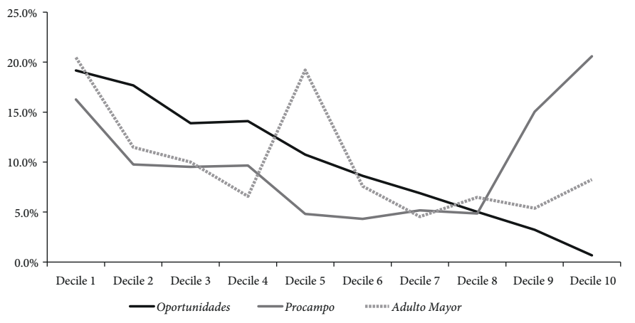
Source: Authors own elaboration with microdata from ENIGH 2008 from INEGI (2009).
Figure 1 Social programs distribution by income decile, 2008
The results of the Absolute simulation are shown in Table 3. The sectors that are most affected are: Apparel Manufacturing, Leather and Allied Product Manufacturing; Accommodation and Food Services; Educational Services; Other Services (except Public Administration) and Utilities. The effect on the gross production of these sectors ranges between -2.96% to -1.92% in the case of Oportunidades, -1.23% to -0.78% for Procampo, and -0.70% to -0.45% for the Adulto Mayor program. Nonpaid workers are the most affected by the elimination of the programs. For Oportunidades, the effects range between -1.63% for nonpaid workers to -1.06% for private capital owners. With respect to Procampo, the impact ranges between -0.64% to -0.43%, and for Adulto Mayor, from -0.38 to -0.25. The most affected households are the low-income deciles. Eliminating Oportunidades reduces income between -5.16% and -1.04%, eliminating Procampo, between -1.84% and -0.55%, and removing Adulto Mayor, between -1.27% and -0.26%.
Table 3 Economic sectors, households, and productive factors most affected in proportion to their income due to the elimination of social programs, Absolute simulation
| Economic sectors | Oportunidades | Procampo | Adulto Mayor |
|---|---|---|---|
| Apparel Manufacturing, Leather and Allied Product Manufacturing | -2.96% | -1.23% | -0.70% |
| Accommodation and Food Services | -2.77% | -1.14% | -0.65% |
| Educational Services | -2.67% | -1.18% | -0.64% |
| Other Services (except Public Administration) | -2.21% | -0.96% | -0.53% |
| Utilities | -1.92% | -0.78% | -0.45% |
| Primary factors | |||
| Nonpaid worker | -1.63% | -0.64% | -0.38% |
| Employer | -1.29% | -0.52% | -0.30% |
| Self-employed | -1.23% | -0.49% | -0.29% |
| Employee | -1.18% | -0.49% | -0.28% |
| Capital | -1.06% | -0.43% | -0.25% |
| Households | |||
| Decile 1 | -5.16% | -1.84% | -1.27% |
| Decile 2 | -3.65% | -0.99% | -0.63% |
| Decile 3 | -2.40% | -0.80% | -0.47% |
| Decile 4 | -2.20% | -0.74% | -0.36% |
| Decile 5 | -1.76% | -0.55% | -0.55% |
| Decile 6 | -1.52% | -0.52% | -0.34% |
| Decile 7 | -1.39% | -0.53% | -0.30% |
| Decile 8 | -1.24% | -0.50% | -0.30% |
| Decile 9 | -1.13% | -0.59% | -0.28% |
| Decile 10 | -1.04% | -0.50% | -0.26% |
Source: Authors’ own elaboration.
The numbers are cold and might not express in the right dimension the consequences of aborting these social programs. If the burden of the income contraction of the first decile under the Absolute scenario were experienced by the 20% poorest households of the first decile, that would represent an income cut of 56%; if it were levied on the poorest ones, that would be equivalent to leaving 223,000 families without any income.
In the short term, the elimination of social programs and the allocation of resources to pay the debt has a negative impact on the country’s gross value added of 0.94% due to the elimination of the Oportunidades program, of 0.38% for Procampo and 0.22% for the Adulto Mayor Program.
We consider the scenario where the released resources of the eliminated social programs are transferred back to the families according to the current labor income tax burden, what we call the Net scenario. Because the programs, especially Oportunidades and Adulto Mayor, are concentrated in the low-income deciles, whereas 83.50% of the labor income tax is concentrated in the three highest income deciles, this policy combination generates initial positive net impacts for households in deciles 7 to 10 and initial negative impacts for households from deciles 1 to 6.
Table 4 shows the main outcomes of the simulation under the Net scenario. The sectors presenting the largest percentual contractions are Agriculture, Forestry, Fishing and Hunting; Food Manufacturing; Beverage and Tobacco Product Manufacturing; Transportation and Warehousing; Wholesale and Retail Trade; and Paper Manufacturing, and Printing and Related Support Activities. Those sectors that benefited the most are Educational Services; Information; Arts, Entertainment, and Recreation; Other Services (except Public Administration); and Health Care and Social Assistance. Note that deciles 1 to 6 have high marginal propensities to consume in the goods and services sold by the affected sectors, and deciles 7 to 10 in the goods and services sold by the benefited sectors. Most of the productive factors are negatively affected, except for employees, who benefit under this scenario. As the initial shock dictates, the households that benefit are the richest ones, from deciles 7 to 10. In the aggregate, under this scenario the effect on gross value added is practically zero.
Table 4 Economic sectors, households, and productive factors most affected in proportion to their income due to the elimination of social programs under the Net simulation
| Economic sectors | Oportunidades | Procampo | Adulto Mayor |
|---|---|---|---|
| Agriculture, Forestry, Fishing and Hunting | -0.54% | -0.14% | -0.11% |
| Food Manufacturing | -0.40% | -0.10% | -0.08% |
| Beverage and Tobacco Product Manufacturing | -0.18% | -0.05% | -0.03% |
| Transportation and Warehousing | -0.17% | -0.04% | -0.03% |
| Wholesale and Retail Trade | -0.11% | -0.02% | -0.02% |
| Paper Manufacturing, Printing and Related Support Activities | -0.11% | -0.03% | -0.02% |
| Health Care and Social Assistance | 0.25% | 0.06% | 0.05% |
| Information | 0.30% | 0.07% | 0.06% |
| Arts, Entertainment, and Recreation | 0.36% | 0.09% | 0.07% |
| Other Services (except Public Administration) | 0.38% | 0.10% | 0.07% |
| Educational Services | 0.60% | 0.15% | 0.12% |
| Primary factors | |||
| Nonpaid worker | -0.16% | -0.04% | -0.03% |
| Employer | -0.05% | -0.01% | -0.01% |
| Self-employed | -0.05% | -0.01% | -0.01% |
| Capital | -0.03% | -0.01% | -0.01% |
| Employee | 0.09% | 0.02% | 0.02% |
| Households | |||
| Decile 1 | -4.31% | -1.49% | -1.07% |
| Decile 2 | -2.71% | -0.61% | -0.41% |
| Decile 3 | -1.37% | -0.37% | -0.23% |
| Decile 4 | -1.10% | -0.29% | -0.10% |
| Decile 5 | -0.55% | -0.06% | -0.27% |
| Decile 6 | -0.25% | 0.00% | -0.04% |
| Decile 7 | 0.04% | 0.05% | 0.04% |
| Decile 8 | 0.24% | 0.07% | 0.04% |
| Decile 9 | 0.47% | 0.10% | 0.10% |
| Decile 10 | 0.48% | 0.12% | 0.10% |
Source: Authors’ own elaboration.
4.2. Mexico’s social programs impact on poverty: An extraction simulation
Employing the microdata of the ENIGH 2008 (INEGI, 2009) we estimate the FGT poverty indexes for α = 0, 1 and 2. Besides, using the consumption per adult equivalent distribution, a Lorenz Curve was fitted employing ordinary least squares following Kakwani (1980), and the second derivative of this curve at the head count measure of poverty was estimated to infer the density evaluated at the poverty line. With all these inputs we are able to estimate the poverty elasticities regarding mean income and Gini coefficient, presented in Table 5.
Table 5 Estimated poverty elasticities to mean income and Gini coefficient in Mexico, 2008
| Α | FGT poverty indexes | Elasticities | |
|---|---|---|---|
| Income | Distribution | ||
| 0 | 0.1283 | -2.0873 | 4.6802 |
| 1 | 0.0407 | -2.1535 | 10.4965 |
| 2 | 0.0188 | -2.3324 | 15.0465 |
Source: Authors’ own elaboration.
Using the initial and simulated incomes, the Gini coefficient of the income distribution, and the poverty elasticities, we arrive to estimates of the percentual increase in the poverty indexes due to eliminating the social programs. Table 6 presents the main results of the impact of the three social programs, one program at a time under both scenarios. Annual mean income and Gini coefficients are reported, as well as the estimated percentual variations in poverty due to the income and inequality changes, and the total effect. As it is natural, the decrease in mean income is larger for the Absolute than for the Net scenarios because in the latter the elimination of the social programs’ cash transfers is compensated with tax rebates for the rest of the families, hence the net effect dilutes. The Net scenario presents the major increases in the Gini coefficient, because the simulation takes money from the poorest families and transfer it to the highest income families. For this reason, the income effect on the FGT poverty measures is more important in the Absolute scenario and the distribution effect is more relevant in the Net simulation.
Table 6 Estimated percentual increase in poverty indexes because of the extraction of the social programs under the Absolute and Net scenarios
| Oportunidades | Procampo | Adulto Mayors | |||||
|---|---|---|---|---|---|---|---|
| Benchmark | Absolute | Net | Absolute | Net | Absolute | Net | |
| Mean income | 368,692 | 363,437 | 368,689 | 366,548 | 368,695 | 367,464 | 368,691 |
| Gini coefficient | 0.4833 | 0.4865 | 0.4873 | 0.4840 | 0.4844 | 0.4839 | 0.4841 |
| Income effect | |||||||
| α = 0 | 0.0297 | 0.0000 | 0.0121 | 0.0000 | 0.0070 | 0.0000 | |
| α =1 | 0.0307 | 0.0000 | 0.0125 | 0.0000 | 0.0072 | 0.0000 | |
| α = 2 | 0.0332 | 0.0000 | 0.0136 | 0.0000 | 0.0078 | 0.0000 | |
| Distribution effect | |||||||
| α = 0 | 0.0306 | 0.0389 | 0.0065 | 0.0101 | 0.0058 | 0.0078 | |
| α = 1 | 0.0687 | 0.0873 | 0.0147 | 0.0226 | 0.0129 | 0.0174 | |
| α = 2 | 0.0985 | 0.1252 | 0.0210 | 0.0324 | 0.0185 | 0.0250 | |
| Total effect | |||||||
| α = 0 | 0.0604 | 0.0389 | 0.0187 | 0.0100 | 0.0127 | 0.0078 | |
| α = 1 | 0.0994 | 0.0873 | 0.0272 | 0.0226 | 0.0201 | 0.0174 | |
| α = 2 | 0.1318 | 0.1252 | 0.0346 | 0.0323 | 0.0263 | 0.0250 | |
Source: Authors’ own elaboration.
Oportunidades is clearly the program with the largest impact in the FGT poverty indexes. Cancelling the program means a rise in the poverty indexes from 6.04 to 13.18 percent, depending on the definition of poverty in the Absolute scenario, whereas eliminating Procampo rises poverty in a range of 1.87 to 3.46 percent, and 1.27 to 3.63 for the Adulto Mayor program. The differential impact might be explained because Procampo weakly targets poverty and the Adulto Mayor program is relatively new and with smaller budgets, compared to Oportunidades.
In all cases the distribution effect runs in the same direction as the income effect, that is, the first reinforces the second. In the case of the incidence of poverty or the head count index, both effects are roughly of the same magnitude. In the case of Oportunidades, the contraction of the mean income of the poor, directly by the cash transfer and indirectly by the multiplier effects in the SAM model, produce a rise in poverty of the same size than the one produced by the increase in the Gini coefficient. Rises in poverty under the Net scenario are due almost entirely to the distribution effect.
Let assess the contribution of the social programs on poverty incidence. Our extraction exercise in the Absolute scenario leads us to conclude that the proportion of households in poverty would increase 9.18% if all three social programs were eliminated. As in 2008 the head count poverty in Mexico was 12.83%, then poverty incidence would rise to 14.01%, an increase of 1.21 percentual points, meaning 1.4 million more poor individuals in the economy.
Is the impact of the three programs in terms of poverty alleviation small or large? Clearly the alleviation of poverty of the social programs considered is not minor, but it can be insufficient depending on Mexico’s goals and its commitments regarding poverty. It is difficult to establish a desired goal for poverty in the next decade for Mexico but let us advance two possible goals: The first one is to accomplish the parameters established in the Sustainable Development program of the World Bank that pretends to eradicate extreme poverty by 2030; the second is to drop poverty incidence to levels compatible with the degree of Mexico´s development.
According to the World Bank’s parameters, then every household should have an income to afford at least 1.25 US dollars per person per day3. In 2008, poverty line in Mexico was approximately 805.1 pesos monthly and the 1.25 US dollars line was equivalent to 417.35 pesos, then under a uniform distribution, making all population having an income greater than the World Bank poverty line is equivalent to reduce the poverty incidence in Mexico by 52%.
The second standard also implies a huge drop in the poverty incidence in Mexico. Taking 71 country observations of World Bank extreme poverty incidence estimations and Gross Domestic Product (GDP) per capita, we estimate that according to their per capita income level, Mexico’s poverty incidence should be 50% lower compare with its actual level4. In order of magnitude, both standards point to a goal of dropping the poverty incidence in Mexico by half in the next decades.
Our results indicate that to achieve such a reduction, the social programs should be increased by a factor of 8 if they remain as they operate. Some gains might be achieved changing the rules of operation in the case of Procampo and making sure the transfers from Oportunidades and Adulto Mayor programs trickle down to the first and second decile of the income distribution. Although, even in this scenario, the amount of resources devoted to alleviating poverty should increase dramatically to cut poverty in Mexico by half.
5. Conclusions
The cancellation of social programs Oportunidades, Procampo and Adulto Mayor would affect the lowest income deciles and the following economic sectors: Apparel Manufacturing; Leather and Allied Product Manufacturing; Accommodation and Food Services; Educational Services; Other Services (except Public Administration); and Utilities. If the budget was destined to pay debt, it would have a negative effect on the country’s gross value added, in the Oportunidades program a decrease of 0.94%, 0.38% for Procampo and 0.22% for the Adulto Mayor program.
If the three programs were canceled at the same time, the poverty rate would increase 9.18%, based on 2008, and the poverty head-count rate would go from 12.83% to 14.01%, which represents 1.4 million poor individuals additionally. Moreover, based on this extraction experiment, we infer that reducing poverty to the levels required by the 2030 World Bank's goals, it would be necessary to scale up the budget for these social programs by a factor of 8.
Our research shows that the macro-outcomes of poverty or social programs must consider the income distribution effect of public policies on poverty, especially when we employ realistic scenarios where the employed resources in these programs are funded by taxpayers. However, it should be noted that measuring the impact through removing a program may be generally different from the effect of implementing it for the first time. The behavior of agents changes once they incorporate the resources they receive into their endowment, hence when they lose them the behavioral reaction may be different compared with when they first received them. This important methodological consideration is not approached in our model; it is left for further research.
A broader scope of the transmission mechanisms of these social programs can be achieved allowing for relative prices flexibility because the extraction of the considered social programs in Mexico might alter the relative prices of the production factors if their supplies are inelastic. A natural extension of the model is to incorporate a less restrictive assumption about the supply price elasticities.
In the public policy arena, the exercise shows that anti-poverty programs in Mexico, such as Oportunidades, have a significant effect on poverty alleviation. However, the exercise brings into question if they can reduce poverty any further. More work is needed to make a complete assessment about the possibilities of these type of programs in achieving a steady state poverty rate compatible with the World Bank and United Nations goals, based on a natural growth rate of the gross domestic product of just 2%, which has been the average growth in the last twenty years. To explore this issue, we need to develop a dynamic general equilibrium model, an effort that is beyond the purpose of this paper.
Finally, social programs such as Oportunidades, Adulto Mayor and Procampo are subject to important changes in the Lopez Obrador administration. Oportunidades became an unconditional scholarships program, the Adulto Mayor program was re-launched increasing substantially the transfers to all Mexicans above 65 years old independently if they receive or not a contributive pension from a social security institution, and Procampo has been partially replaced by a minimum price on traditional crops. Under these circumstances, we consider our study contributes to the debate about how to design social programs to combat poverty efficiently.

