


 nueva página del texto (beta)
 Inglés (pdf)
 Artículo en XML
 Referencias del artículo
 Enviar artículo por email
 Citado por SciELO
  Similares en
SciELO
Similares en
SciELO 
 Permalink
1. INTRODUCTION
The near-linear character of the price rate of profit (PRP) trajectories and wage rate profit (WRP) curves have been too old and still puzzling empirical regularities that were ascertained in the research following the famous Cambridge Capital Controversies (CCC) of the 1960s. The controversies were about the measurement of capital in a way consistent with the tenets of the neoclassical theory, according to which the prices of factors of production reflect their respective relative scarcities. A hypothesis that the CCC have shown that it does not necessarily hold (Tsoulfidis, 2010, ch. 8 and the literature cited there). More specifically, economists mainly from the Cambridge UK side showed that the relative scarcity of capital may be associated with a lower rate of profit orvice versa; hence, we may have the case of reverse capital deepening phenomenon. Furthermore, a capital-intensive technique may be selected at both lower and higher rates of profit, whereas in the middle range of the rate of profit, the labor-intensive technique is to be selected. In general, the economists from the Cambridge UK side, inspired by Sraffa’s (1960) contributions, argued that the “capital intensity” is an endogenous variable depending on income redistribution and the resulting complexities in price movements may change the characterization of an industry from capital to labor-intensive and vice versa.
Samuelson (1962) from the neoclassical side responded to these critiques by utilizing a surrogate model of an economy producing a single commodity and derived results seemingly consistent with the neoclassical theory of value. This parable production function model was criticized for its lack of realism, simply because in such a model there are no prices, and so the capital-intensity is not affected by changes in income distribution. Levhari (1965) responded to these critiques by arguing that reswitching is not possible in the case where the matrix of technological coefficients is indecomposable. However, not long after, Levhari and Samuelson (1966) and Samuelson himself (1966) admitted the presence of reswitching and, therefore, the remaining inconsistency in the core of the neoclassical theory of value.
Sraffians, at that time, did not have to offer any fully worked-out alternative to the neoclassical economics model, but only the foundations to build one. The weaknesses in the Sraffian and the classical approach might partially explain why neoclassical economists continued to hold to their theory, despite acknowledging its inconsistency. However, this should not be interpreted to mean that neoclassical economics was not affected at all by the CCC. On the contrary, the CCC influenced the direction of economic theory by far more than is usually recognized. In the years following the CCC, neoclassical economists started engaging more intensively in the intertemporal general equilibrium approach. The latter seems to have escaped the capital theory critique simply because in this approach there are only commodity flows delivered at different times and, therefore, there are no capital and stock variables, in general. According to the intertemporal approach, there is no need to theorize a general rate of profit. Consequently, this strand of neoclassical economics also dispenses with the long-period method of analysis shared by both classical and the standard neoclassical theories.
From the Sraffian and the broader classical approach, we had had the further development of the linear models of production and the utilization of input-output data in the estimation of equilibrium prices. More specifically, Krelle (1977) from the neoclassical side, using input-output data from West Germany, showed that the WRP curves (of the years 1958, 1960, 1962, and 1964) were quasi-linear, thereby casting doubt on the claims to the reswitching scenarios of the Sraffian economists. Ochoa (1984; 1989) and Shaikh (1984; 1998) using complete data sets for the US economy and the benchmark years 1947, 1953, 1958, 1967, and 1972, confirmed the near-linear character of both the WRP curves and the PRP trajectories. These results are not in line with Sraffa’s conjecture of complexities in PRP paths and WRP curvatures induced by changes in income distribution. It is equally important to stress at this point that the near-linearity of the WRP curves does not lend support to neoclassical economics either because they do not point to any causal relationship running from marginal productivities of factors of production to their respective payments.
These first empirical studies took a long time to attract the attention they deserved from both sides of the debate. The neoclassical economists were no longer interested in issues of capital theory, especially after the disappointing outcome of the debates for their theory. The Sraffians, on the other hand, downplayed the importance of the empirical findings. For example, Kurz and Salvadori (1995, p. 450) opined that the empirical tests by hypothesizing that the choice is always from the available techniques in just a single year and country and, in so doing, other available techniques were not considered. Han and Schefold (2006), in their effort to account for all possible techniques between pairs of countries and intertemporal, found rare occasions of reverse capital deepening or reswitching. Zambelli, Fredholm, and Venkatachalam (2017) found that although WRP curves are near-linear, there is nevertheless capital reversing and reswitching only for unrealistic rates of profit, ranging between 60% and 250%. In the face of this evidence, Kurz (2020) argued that the quality of the available data was an additional obstacle to deriving definitive results and conclusions. The empirical research has shown what was expected, the more complete the data the more favorable the results concerning linearities. On the other hand, in the intertemporal comparisons, if the years are not far from each other, say five years, as in the research for the US economy, all available techniques, one way or another, are accounted. For example, starting with the techniques of the year 2012 forming the economy-wide average near-linear WRP curve, these same techniques, most likely, were available also in the benchmark year 2007, but only to fewer firms weighing by far less in the estimated quasi-linear WRP curve of 2007.
Thus, if in every year tested the derived WRP curves are quasi-linear (e.g., Ochoa, 1989, Shaikh, 2016; Tsoulfidis, 2021); there is no reason, whatsoever, to suppose there are other techniques in the economy characterized by wide curvatures that may give rise to reswitching and reverse capital deepening and have been ignored. Several studies not only ascertain the near-linearity character of the PRP trajectories and the near-linearity WRP curves and the associated with these frontiers but additionally they offer explanations varying from the closeness of vertically integrated compositions of capital between sectors (Shaikh, 1984; Petrović, 1991; Torres-González, 2020; Torres-González and Yang, 2019) and the nearly randomly distributed input-output coefficients (Bródy, 1997; Schefold, 2013, 2020).
In this article, we follow a different route in which the low effective-rank of the system matrices shapes the exponential fall in their eigenvalues, which in turn determines the near-linearity of PRP and WRP curves (Mariolis and Tsoulfidis, 2009, 2011, 2014, 2016a, 2016b, and 2018). Hence, the specific shapes of the PRP paths and WRP curves are strictly connected to this exponential fall of eigenvalues and the associated with this fall notion of effective rank. The direct and reliable estimation of the latter is quite challenging. For this reason, we propose an indirect method to estimate the effective rank of the economy’s matrix through an eigendecomposition of the prices of production into a polynomial expression. The number of required terms of such an eigendecomposition for a satisfactory approximation to prices is what dictates the effective rank of the matrix, which proves to be by far lower than its numerical (nominal) one.
The remainder of the article is structured as follows: Section 2 presents the preliminaries for the estimation of the direct prices (DP) and prices of production (PP), as well as their possible trajectories as an effect of income redistribution. Section 3 presents and critically evaluates the estimates of DP and PP derived by using the benchmark input-output table of the US economy for the year 2012. Section 4, using the same data set, subjects to empirical testing the randomness hypothesis. Section 5 deals with the near-linear character of the price trajectories and by suggesting their dimensionality reduction through an eigendecomposition. Subsequently, these trajectories are approximated by linear, quadratic, cubic, or even higher-order terms of the resulting factorization. Section 6 concludes with a summary and suggestions for future research efforts.
2. DIRECT PRICES, PRICES OF PRODUCTION AND CAPITAL INTENSITIES
We start with the application of a circulating capital model and input-output data of the US economy of the year 2012, the last available benchmark year. The results ascertain the near-linear character of the PRP trajectories and the WRP curve of the US economy.
We begin with the labor values, which are estimated through the following equation:
where upper-case bold-faced letters refer to square matrices, lower-case bold-faced letters refer to vectors of dimensions conformable to pre- or post-multiplication by matrices; finally, scalars are indicated by lower case letters in italics. The notation in equation [1] is as follows: λ = 1(n vector of prices of unit values λ; l = 1(n vector of employment coefficients; A = n(n matrix of input-output coefficients; D = n(n matrix of depreciation coefficients2; I = n(n identity matrix of the same dimensions with the matrix A.
The labor values or, what is the same, the vertically integrated employment coefficients are estimated from:
The vector of unit labor values λ is normalized through its multiplication by the monetary expression of labor time (MELT), which in our case is the ratio of the column vector of gross output x, evaluated at market prices (MP) denoted by the row vector e, over the same gross output vector evaluated in unit labor values (λx). Thus, the monetary expression of labor values called ‘direct prices’ (Shaikh, 1984; 1998) and symbolized by v are defined as follows:
The vector of PP is estimated from the following equation:
where r = the economy-wide rate of profit; b = nx1 vector of the basket of goods that workers purchase with their money wage, w; π = 1xn left hand side vector, the only positive corresponding to the maximal eigenvalue, r -1, and it is defined up to multiplication by a scalar. < t > = nxn diagonal matrix of the net of subsidies indirect taxes per unit of output3.
Equation [3] is transformed to the following eigenequation:
The estimated unique left-hand side relative prices are normalized by a Sraffian type of standard commodity σ derived from the right-hand side eigenvector of the matrix:
We set H = A[I - A - D - < t>]-1 and so the above equation is rewritten as:
where
The next step is to fix the relative prices by the normalized standard commodity, s, and derive the normalized row vector of PP, p:
and in so doing (see Shaikh, 1998), we establish the following equalities
Thus, equation [4] can be rewritten as:
where w = pb the money wage, which is equal to the value of basket of commodities purchased by workers. We post-multiply equation [6] by the normalized standard commodity and we get:
It follows that:
We divide through by vs and we end up with:
which solves for the linear WRP curve:
where ρ ≡ rR-1, with 0 ≤ ρ ≤ 1. By substituting in equation [6], we arrive at:
We know that the maximum eigenvalue of the matrix H R equals to one and, therefore, the matrix H Rρ has an eigenvalue less than one, which is equivalent to saying that the so-derived matrix becomes convergent. Hence, the matrix H represents the vertically integrated input-output matrix. From the above, it follows that ‘Sraffa’s conjecture’ for the development of quite complex price-feedback effects, because of income redistribution so strong as to change the characterization of industries from capital- to labor-intensive and vice versa, is certainly a theoretical possibility deserving further investigation of the conditions that give or do not give rise to that.
3. PRICE TRAJECTORIES USING INPUT-OUTPUT DATA OF BEA 2012
Before we start with the plotting of trajectories of PP relative to DP, it is important to show the proximity of DP and PP to each other and to MP using both circulating and fixed capital models and also the respective industry capital-intensities relative to the standard ratios and the related statistics of dispersion. Thus, the first column in Table 1 below presents the DP while the next two columns present the PP for the circulating and fixed capital models, respectively. The Mean Absolute Deviation (MAD) computed as the mean value market of the absolute difference of estimated prices relative to MP, which by definition are equal to one million dollars’ worth of output (see Miller and Blair, 2009, ch. 2) and so the MP are equal to the row (1×70) vector of ones. The Mean Absolute Weighted Deviation (MAWD) multiplies the row vector of the absolute differences of the two prices relative to MP times the column vector of each industry’s share in total output. In the same spirit and independent of the chosen numéraire the
Table 1 Direct prices, prices of production and capital-intensities, BEA 2012
| Industries | DP | PP circulating capital | PP fixed capital | Circulating capital-intensity, 1/R = 1.4 | Fixed capital-intensity / R = 3.02 | |||
| 1 | Farms | 0.749 | 0.880 | 0.863 | 2.159 | 7.697 | ||
| 2 | Forestry, fishing, and related activities | 1.062 | 0.938 | 0.902 | 0.889 | 2.759 | ||
| 3 | Oil and gas extraction | 0.862 | 0.960 | 1.140 | 1.683 | 9.559 | ||
| 4 | Mining, except oil and gas | 0.824 | 0.905 | 0.840 | 1.753 | 5.121 | ||
| 5 | Support activities for mining | 0.888 | 0.801 | 0.764 | 1.053 | 3.118 | ||
| 6 | Utilities | 0.750 | 0.852 | 1.087 | 1.637 | 11.168 | ||
| 7 | Construction | 0.963 | 0.893 | 0.784 | 1.152 | 2.398 | ||
| 8 | Wood products | 1.027 | 1.072 | 0.892 | 1.668 | 3.153 | ||
| 9 | Non-metallic mineral products | 0.985 | 0.996 | 0.896 | 1.504 | 3.820 | ||
| 10 | Primary metals | 0.931 | 1.084 | 0.875 | 2.135 | 4.203 | ||
| 11 | Fabricated metal products | 1.020 | 1.049 | 0.871 | 1.586 | 3.014 | ||
| 12 | Machinery | 1.012 | 1.064 | 0.862 | 1.691 | 2.928 | ||
| 13 | Computer and electronic products | 1.173 | 1.027 | 0.998 | 0.936 | 2.966 | ||
| 14 | Electrical equipment, appliances, etc. | 1.005 | 1.017 | 0.848 | 1.529 | 2.892 | ||
| 15 | Motor vehicles, bodies & trailers | 0.998 | 1.194 | 0.878 | 2.263 | 3.276 | ||
| 16 | Other transportation equipment | 1.012 | 1.002 | 0.830 | 1.474 | 2.522 | ||
| 17 | Furniture and related products | 1.088 | 1.121 | 0.924 | 1.605 | 2.908 | ||
| 18 | Miscellaneous manufacturing | 1.006 | 0.971 | 0.844 | 1.316 | 2.758 | ||
| 19 | Food, beverage and tobacco | 0.819 | 1.032 | 0.825 | 2.388 | 4.933 | ||
| 20 | Textile mills and textile product mills | 1.024 | 1.112 | 0.949 | 1.776 | 4.030 | ||
| 21 | Apparel and leather and allied products | 1.233 | 1.135 | 1.015 | 1.116 | 2.516 | ||
| 22 | Paper products | 0.968 | 1.078 | 0.890 | 1.920 | 3.913 | ||
| 23 | Printing and related support activities | 1.035 | 1.007 | 0.896 | 1.339 | 3.189 | ||
| 24 | Petroleum and coal products | 0.759 | 0.986 | 0.951 | 2.519 | 8.601 | ||
| 25 | Chemical products | 0.820 | 0.953 | 0.823 | 2.043 | 5.072 | ||
| 26 | Plastics and rubber products | 0.941 | 1.041 | 0.854 | 1.869 | 3.745 | ||
| 27 | Wholesale trade | 0.843 | 0.838 | 0.802 | 1.180 | 3.451 | ||
| 28 | Motor vehicle and parts dealers | 0.998 | 0.993 | 1.012 | 0.957 | 3.801 | ||
| 29 | Food and beverage stores | 1.024 | 0.978 | 1.034 | 1.019 | 4.618 | ||
| 30 | General merchandise stores | 1.045 | 1.067 | 1.086 | 1.052 | 4.038 | ||
| 31 | Other retail | 0.919 | 0.918 | 0.986 | 1.133 | 5.285 | ||
| 32 | Air transportation | 0.895 | 0.993 | 0.929 | 1.679 | 4.985 | ||
| 33 | Rail transportation | 1.008 | 0.947 | 1.108 | 1.244 | 7.188 | ||
| 34 | Water transportation | 1.042 | 1.088 | 0.974 | 1.749 | 4.366 | ||
| 35 | Truck transportation | 0.987 | 0.988 | 0.886 | 1.438 | 3.582 | ||
| 36 | Transit and ground pass. Transportation | 0.819 | 0.713 | 0.699 | 0.864 | 2.909 | ||
| 37 | Pipeline transportation | 0.782 | 0.765 | 1.023 | 1.220 | 9.852 | ||
| 38 | Other transport. and support activities | 1.055 | 0.967 | 0.889 | 1.130 | 2.914 | ||
| 39 | Warehousing and storage | 1.055 | 1.005 | 1.069 | 1.293 | 5.715 | ||
| 40 | Publishing, except internet | 0.979 | 0.850 | 0.830 | 0.949 | 3.020 | ||
| 41 | Motion picture and recording industries | 0.932 | 0.888 | 0.952 | 1.177 | 5.298 | ||
| 42 | Broadcasting and telecommunications | 0.835 | 0.853 | 0.874 | 1.513 | 5.719 | ||
| 43 | Data processing, internet publishing, etc. | 0.914 | 0.887 | 0.820 | 1.417 | 3.709 | ||
| 44 | Fed., credit intermediation, etc. | 0.847 | 0.740 | 0.756 | 0.956 | 3.670 | ||
| 45 | Securities, commodity contracts, etc. | 1.206 | 1.034 | 0.991 | 0.951 | 2.692 | ||
| 46 | Insurance carriers and related activities | 0.888 | 0.829 | 0.734 | 1.204 | 2.422 | ||
| 47 | Funds, trusts, and other financial vehicles | 1.019 | 1.089 | 0.889 | 2.026 | 3.378 | ||
| 48 | Other real estate | 1.131 | 1.174 | 2.376 | 1.612 | 23.305 | ||
| 49 | Rental and leasing services etc. | 0.722 | 0.747 | 0.766 | 1.540 | 5.816 | ||
| 50 | Legal services | 0.874 | 0.741 | 0.757 | 0.793 | 3.160 | ||
| 51 | Computer systems design etc. | 1.126 | 0.871 | 0.828 | 0.530 | 1.318 | ||
| 52 | Miscellaneous professional, scientific, etc. | 1.032 | 0.862 | 0.850 | 0.808 | 2.711 | ||
| 53 | Management of companies and enterprises | 1.237 | 1.010 | 1.016 | 0.705 | 2.626 | ||
| 54 | Administrative and support services | 1.103 | 0.903 | 0.845 | 0.731 | 1.782 | ||
| 55 | Waste management and remedy services | 0.986 | 0.953 | 0.905 | 1.276 | 3.805 | ||
| 56 | Educational services | 1.151 | 0.963 | 1.090 | 0.735 | 4.588 | ||
| 57 | Ambulatory health care services | 1.116 | 0.913 | 0.901 | 0.721 | 2.477 | ||
| 58 | Hospitals | 1.193 | 1.022 | 1.020 | 0.886 | 3.167 | ||
| 59 | Nursing and residential care facilities | 1.221 | 1.041 | 1.076 | 0.814 | 3.491 | ||
| 60 | Social assistance | 1.192 | 1.029 | 1.039 | 0.906 | 3.485 | ||
| 61 | Perform. arts, spectator sports, museums | 0.863 | 0.776 | 0.827 | 0.958 | 4.372 | ||
| 62 | Amusements, gambling, and recreation | 0.922 | 0.871 | 0.945 | 1.020 | 5.072 | ||
| 63 | Accommodation | 0.921 | 0.912 | 0.939 | 1.154 | 4.655 | ||
| 64 | Food services and drinking places | 1.015 | 0.979 | 0.960 | 1.178 | 3.969 | ||
| 65 | Other services, except government | 1.051 | 0.917 | 0.943 | 0.879 | 3.648 | ||
| 66 | Federal general government (defense) | 1.149 | 1.002 | 0.996 | 0.979 | 3.458 | ||
| 67 | Federal general government (nondefense) | 1.190 | 0.988 | 1.091 | 0.798 | 4.325 | ||
| 68 | Federal government enterprises | 1.635 | 1.328 | 1.620 | 0.838 | 6.050 | ||
| 69 | State and local general government | 1.260 | 1.021 | 1.172 | 0.678 | 4.584 | ||
| 70 | State and local government enterprises | 1.097 | 0.989 | 1.270 | 1.230 | 8.737 | ||
| Mean absolute deviation | 0.112 | 0.084 | 0.140 | SD | 0.456 | SD | 2.974 | |
| Mean absolute weighted deviation | 0.130 | 0.086 | 0.171 | Mean | 1.299 | Mean | 4.507 | |
| d-statistic | 0.150 | 0.112 | 0.228 | CV | 0.351 | CV | 0.660 | |
The last two columns of Table 4.1 stand for the vertically integrated capital-intensities of industries in circulating and fixed capital models, respectively. The estimations of capital-intensities in both models are at a relative rate of profit equal to zero and so PP = DP = MP. This gives us an initial grasp of the deviations between capital-intensities at the starting point of the trajectories of PPs. The standard ratios are also reported in the top two right cells of Table 1 and they are equal to 1.414 and 3.017 for circulating and fixed capital models, respectively. The standard deviations and the mean of these capital-intensities are displayed in the last two rows of the Table. The coefficient of variation in the fixed capital model is nearly twice higher than that of the circulating capital model. This outcome alone makes more unlikely the case of crossing the PP-DP line of equality by the PP in the fixed capital model in which PP are expected to move monotonically to the upward or downward direction according to their capital-intensity relative to the standard ratio, R. In our case, since the fixed capital matrix is the result of a multiplication of the column vector of investment shares times the row vector of capital-output ratio (see Appendix for more details) its rank is equal to one and of rank one is also the product of the matrix of capital stock times the Leontief inverse augmented by the depreciation matrix and indirect tax coefficients. The PRP trajectories derived with the so estimated capital stock matrix will be straight lines pointing to the upward or downward direction depending on their vertical integrated capital-intensity relative to the standard ratio.
Having established the proximity of DP and PP (in both circulating and fixed capital models) to MP the next step is to show the trajectories of PP in the face of changes of the relative rate of profit, ρ ≡ rR -1. We restrict the analysis to PP in the circulating capital model precisely because that price trajectories in the fixed capital model will be, by definition, straight lines. The WRP curve though will be convex with higher curvature than that of the circulating capital model, whose concave shape is characterized by a light curvature not very different from a straight line. The WRP curves are estimated from equation [6] which we post multiply by x and by invoking our normalization condition vx = px = ex, we arrive at the WRP relation:
We replace ρ ≡ rR -1 and we get for ρ = 0 the maximum wage rate while for ρ = 1, we get the maximum ρ ≡ rR -1 relative rate of profit, that is, the rate of profit at a wage rate equal to zero. Thus, for 0 ≤ ρ < 1, we can generate the WRP curve of the total economy. Similarly, we derive also the WRP curve in the case of fixed capital model, only this time in the above formula, we replace the matrix A by the K matrix and all other terms remain the same. The WRP curves for the year 2012 are depicted in Figure 1 below. We have also drawn a straight dashed line between the two WRP curves to highlight their curvature.
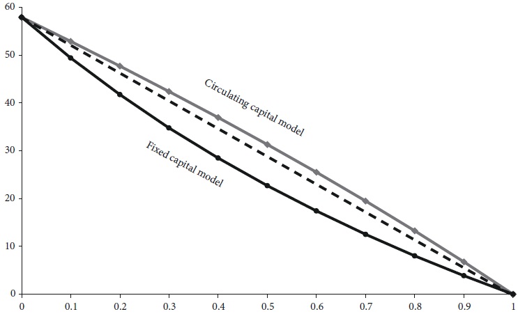
Figure 2 below displays the price trajectories of industries of each and every of our 70 industries for the year 2012 in the circulating capital model4. Hence, we employed equation [8)] and for 0 ≤ ρ < 1 we generated the PP paths relative to DP by applying an element-by-element division of the two vectors for each particular ρ.
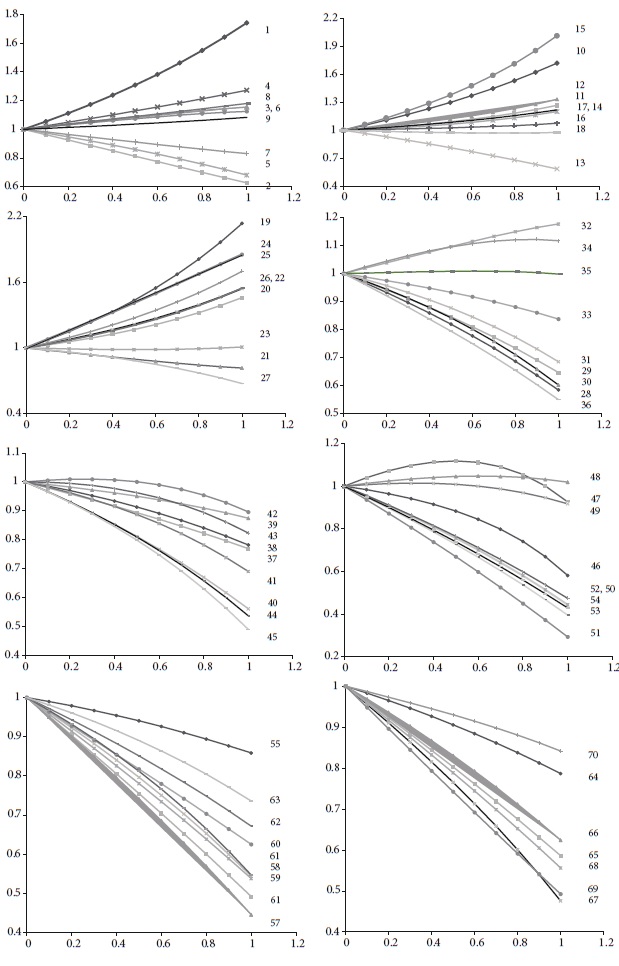
Figure 1 shows that the price trajectories, in most cases, display monotonic behavior, which accelerates (not always) in the upward or downward direction. However, there are eight industries out of seventy with curves displaying a single extreme point, six of which with a maximum (industries 34, 35, 42, 47, 48, and 49) and two with a minimum (industries 18 and 23). It is important to note that these particular industries are characterized by a capital-output ratio closer to the standard as shown in Table 1, enabling the feedback effects at work to exert most of their iMPact on those industries. Furthermore, in all of these industries, although the feedback effects make them display extremes and five of them cross the PP = DP = MP line of equality. Nevertheless, the trajectories of these eight industries remain near the line of equality and display much lower variability than the rest.
In Figure 3 below, we isolate the five industries, whose trajectories cross the line where PP = DP = MP, so as we can take a closer look at them. Although we find extremes and crossings, these crossings occur at distant enough from the equilibrium rate of profit of:
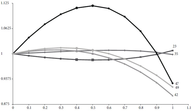
In fact, three industries (23, 35 and 47) cross the line of ones at a relative rate of profit nearly equal or higher than 90%. The other two occurences of crossing still take place at relative rates of profit twice or three times higher than the equilibrium relative rate of profit of 18.8%. Finally, we observe that as the relative rate of profit takes on higher and higher values, the trajectories of PP remain near their DP with a maximum deviation of only 12%. The variability of these PP as measured by their standard deviation with “regular” behavior is the least of all the other industries5.
Despite their non-monotonic movement, the price trajectories of the five industries are too close to the PP = DP = MP line of equality, something that indicates that the capital-intensities of these industries will not be too different from the standard ratio, which is equal to the reciprocal of the maximum eigenvalue 1/R ≈ 1.414.
4. THE CHOICE OF NUMÉRAIRE AND THE RANDOMNESS HYPOTHESIS
The results of the PRP trajectories and WRP curves using as numéraire the gross output vector of the industries, suggest their near linearity. These findings may be challenged as artefacts derived from the possible proximity between the vectors of actual gross output, x, to the standard output, s, which as we show in equation [7] gives a near linear WRP curve. The near-linearity of the WRP curves may be also attributed to the vectors of employment, l, or consumption expenditures coefficients, b, when utilized as numéraires; because both vectors are suspected as being very close to the left-hand side (l.h.s.) and the right-hand side (r.h.s.) eigenvectors of matrix H, respectively (see also Bidard, 2020)6.
For this purpose, we estimate the proximity and strength of association of the vectors of gross output, x, and standard output, s, after their normalization such that their respective column sums to be equal to one. More specifically, we found their MAD = 80.02% whereas the d-statistic = 75.36%. Deviations of this size preclude the proximity of the two vectors as being responsible for the observed near linearities. This does not mean that the two vectors are altogether unrelated; to the contrary, their correlation coefficient is 46.4%.
As for the vectors l and π both normalized in the unit simplex gave a MAD = 82.9% and their d-statistic = 118.7%. The deviations between the two vectors are too large to attribute to them the observed near linearities of PRP trajectories or the WRP curve(s). As in the previous case, we have also found a moderately high correlation coefficient equal to -63.8%, which indicates that the strength of association between the two vectors is quite high. We have also tried the vector of consumption coefficients with the right-hand side eigenvector as suggested by Bidard (2020), but the results were also negative for the closeness of these two vectors.
Of particular interest is the hypothesis of the random character of the matrix A and by extension of the matrix H, as argued initially by Bródy (1997) and recently by Schefold (2013, 2019 and 2020). It is true, that the random matrix hypothesis requires that in the limit all the eigenvalues will be zero or rather trivially small numbers with the exception for the maximal7. However, this pattern of eigenvalues requires random matrices of quite large size, much larger than those usually found in the largest input-output tables. In the hitherto tested input-output tables it has been repeatedly found that the second eigenvalue as well as the third increase, rather than decrease, with the size of the matrix, although they remain sufficiently lower (50 to 60 or even more percent) than the maximal eigenvalue (Mariolis and Tsoulfidis, 2014, 2016a, 2021; Shaikh, Coronado, and Nassif-Pirez, 2020, ch. 6).
Following Schefold (2013, 2019 and 2020) and also his exchange with Mori (2019) and Morioka (2019), the randomness hypothesis requires the following condition: The correlation and covariance coefficients of the difference between the vectors of the gross output and standard output both normalized in the unit simplex, m = x - s, similarly, the difference between the normalized and employment coefficients vector and left-hand side eigenvector vector of the matrix, H, both transposed, n = lʹ - πʹ, should satisfy the following condition:
The intuition behind the above relation is that if x and s are no different from each other it follows that the nearly straight lines in WRP curves may be attributed to the standard output, as shown in relation [7]. In similar fashion if lʹ- πʹ are nearly equal, it follows labor values and prices of production are no different from each other or, what is the same, the capital intensities are the same across industries.
We subjected to empirical testing only the circulating capital model because our fixed capital model by construction has a rank equal to one. Consequently, all eigenvalues except for the first are zero. However, this does not make our capital stock matrix random, because random matrices generically have a full rank, and their eigenvalues may be trivially small, but not necessarily all zero. These characteristics of the fixed capital model imply that the paths of PP will be linear, and the same is true with the capital-output ratios, which we do not show in graphs for reasons of economy in space. The zero subdominant eigenvalues imply that there are absolutely no feedback effects induced by income redistribution on PP, which are strictly linear.
Our data for the year 2012 gave the following correlation coefficient and covariance for the vectors m and n, along with the t-ratio: cor(m,n) = 0.40 with a t-ratio = 3.60 and cov(m,n) = 0.00.
Clearly, the correlation coefficient and the covariance are altogether different; worse than that, the non-zero correlation coefficient, although relatively low is nevertheless statistically significant. The covariance of the two vectors is in this case not different from zero; nevertheless, the covariance is a metric dependent on the units of measurement. Hence, we get zero because the numbers happen to be too small because of the normalization condition. At any rate, since the correlation coefficient is 40% and is statistically significant, it follows that equality between the correlation and covariance cannot hold at zero. Such a result casts doubt if it does not rule out the randomness hypothesis.
5. EIGENDECOMPOSITION, PRICE TRAJECTORIES AND DIMENSIONALITY REDUCTION
We apply what is called eigen- or spectral decomposition, a method of factorization of a matrix into terms consisting of its eigenvalues and eigenvectors. As expected, the first term by virtue of the maximal eigenvalue (provided that the subdominant eigenvalues are by far smaller), exerts most of the influence on PP and their paths and, by extension, on the shape of the WRP curves. Therefore, the idea to identify the number of terms, which are important for a tolerably good approximation of PP and the associated with these eigenvalues or, sometimes, singular values might be useful in our search for the selection of the critical number among the top eigenvalues.
To this end, we invoke the matrix H, which when multiplied by R normalizes the eigenvalues with the maximum being equal to one. Thus, we get the following eigendecomposition form (Meyer, 2001, pp. 517-518; Mariolis and Tsoulfidis, 2018):
where, lambdas, λi , i = 1,2,…,n, stand for the eigenvalues of the matrix H R and y and q are the l.h.s and r.h.s. eigenvectors, respectively. The prime over the vector q indicates its transpose. The first or the maximal eigenvalue is denoted by λ1 = 1, whereas the second eigenvalue by λ2 and the remainder or subdominant eigenvalues by λn . Invoking the Perron-Frobenius theorem, the maximal or dominant eigenvalue is the only one associated with a semi-positive eigenvector uniquely defined when multiplied by a scalar; thus, the first term of the above decomposition will be:
which may be a tolerably good aPProximation of the matrix H, without necessarily referring to the remainder terms (Meyer, 2001, pp. 243-244). The matrix H 1 as the product of two vectors, q 1 y 1, its rank is equal to one and, therefore, it has only one non-zero eigenvalue, the maximal, which by definition is equal to one.
We may test the extent to which the above linear approximation to relative prices, through the first term, H 1, is tolerably good by comparing the trajectories of the resulting PP to those of the actual trajectories. Since the PRP trajectories are not exactly straight lines, the approximation can be improved by adding more of the remaining terms until we reach a point that the approximation no longer improves. If the PRP trajectories are curvy-linear, the first term might make a good approximation indicating a matrix of nominal and effective rank equal to one. In general, though, the number of linearly independent vectors of an actual matrix defines its nominal or numerical rank, which might be considerably higher than its effective rank, especially in cases where the price trajectories are featuring slight curvatures8.
From the above, we arrive at the following steps that need to be taken starting with the presence of quasi-linear price trajectories and PRP curves indicating that the effective rank is significantly smaller than the numerical rank of the matrix A or H estimated at 69 (the sector federal government, defense, has a zero row). Once we establish that only a few terms from the eigendecomposition [10] are enough for a reasonably good approximation, it follows that the effective rank of the system matrices is equal to the number of the utilized terms. Once such an approximation has been carried out, the seemingly complex economies become quite simpler. The low effective rank further indicates that the columns of the estimated matrices are only lightly connected to each other, as there are many zero elements and negligibly small numbers. Consequently, there is pseudo-linear independence between the columns of the matrices under investigation, which amounts to lighter connections between most of the industries, and only a few key industries connect closely to each other and the rest, lending support to the view that the operation of the economy may be captured by only a few sectors. From the above, it follows that the eigendecomposition is the best available alternative to identify the effective rank of matrices. In so doing, we not only simplify the complex structure of the initial matrix, but also we may raise new questions about the properties of the economic system and its structural features.
In Figure 4 below, the lines with the highest curvature are those of the actual trajectories derived from the circulating capital model for the USA (2012) and the matrix H; the straight lines, connecting the start and end-points, are derived from the first term of the above eigendecomposition of the matrix H, that is, the H 1. As a first order approximation, the trajectories of respective relative prices derived from H 1 will be linear while those of H will be curvy, although, in most cases, they are monotonic. It goes without saying that by adding more terms together, the approximation will be, in principle, improving; however, as is the case with meaningful approximations, just a few terms should be adequate. The exact number of the required terms for a satisfactory approximation is determined by the observer's view or the nature of the problem at hand.

In experimenting with the US data of the year 2012 we found that the results derived using the matrix H 1 are quite good. Clearly, the two price trajectories of an industry estimated from H 1 and H coincide at ρ = 0, where the relative PP of the two matrices are equal to each other and to the DP. As ρ increases, the two estimates of relative PP depart from both the DP and themselves moving, in most cases, to the same direction; at the end, that is, when ρ gets to its maximum, the two estimates, that is, the actual relative PP of each and every industry and their respective approximations tend to become equal. In Figure 4 below we display in a panel of eight graphs the trajectories of prices of production of eight industries with their linear and nonlinear approximations. The MAD is displayed on the vertical axis and the ρ is on the horizontal. The eight industries are the ones that display extrema (maximum or minimum points) and, therefore, with the highest curvatures and, at the same time, the lowest variability as measured by their standard deviation. The remaining industries with the higher variability display linearities and so their approximation by higher order terms does not have much to offer.
The five curves displayed in each of the panel of 8 graphs of Figure 4 are as follows: The actual estimated PP is the one with the highest curvature and it is indicated by the dotted solid blue line. The dash-dotted (green) line is the quadratic term with the second eigenvalue equal to 0.479; the cubic term, whose eigenvalue equal to 0.401, is indicated by the dotted (brown) line and finally the fourth or quartic term corresponding to the eigenvalue 0.303 is indicated by the dashed (black) line.
In Figure 5 below, we present estimates of the MAD (vertical axis) between the price trajectories of all our industries and their respective approximations; namely, linear, quadratic, cubic and quartic. The error in each approximation is maximized in the middle range of relative rates of profit shown on the horizontal axis. At ρ = 0.60, the MAD of the linear approximation is 3.243% while at ρ = 0.5 the MAD is slightly lower at 3.236%; of course, the MAD at the start and end points of the curves is zero.
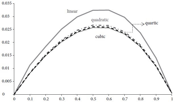
From Figure 5 we observe that the approximation improves moving from the linear to the quadratic term and only slightly improves adding the cubic. The quartic approximation lies between the quadratic and cubic most likely having to do with rounding errors, whose significance increases for we are dealing with small, very small, numbers whose inversion increases the possible rounding errors. In our estimations we got the maximum deviation in the case of the quadratic approximation to occur in industry 47, whose percentage error has reduced to 12.659% and this is for ρ = 0.5. The maximum MAD (for all industries combined) is equal 2.666% for ρ = 0.5. Finally, the quartic term gave results between the quadratic and cubic estimations which are an indication that we no longer need more terms to improve our approximation. Such results are consistent with those reported by Bienenfeld (1988) who argued and confirmed the accuracy of the quadratic approximation (see also Iliadi et al., 2014). In fact, given that the equilibrium ρ ≈ 18.888%, we found that the deviations starting from linear, quadratic, cubic and quartic are: 1.841, 1.541, 1.488 and 1.509, respectively9.
Although these results are derived from the US input-output data of the year 2012, it is reasonable to assume their generality and applicability to other years or the same year of higher dimensions for the USA as well as to other countries. From the above, it follows that the matrices of vertically integrated technological coefficients H that we are typically dealing with, their approximation by linear or quadratic terms is extremely good. This becomes possible precisely because their maximal eigenvalue compresses most of the explanatory content relinquishing some of it for the second eigenvalue. There is very little left to be explained by the distant cubic term and much less, if any at all, for the quartic order term. After all, for reasonable approximations, we do not need to use many terms. The exponential distribution of eigenvalues which is identified in the input-output data of many countries over the years renders our proposed eigendecomposition estimating method of the effective rank reliable.
6. SUMMARY AND CONCLUSIONS
In this article, we grappled with the old and common to both classical and neoclassical approaches issue of the movement of prices induced by changes in income distribution. And in so doing, we are subjecting to empirical testing the extent to which ‘Sraffa’s conjecture’, namely, the direction of price movements induced by changes in income distribution are both complex and indeterminate. We experimented with the last benchmark input-output table of the US economy of the year 2012 and we found that prices, more often than not, move monotonically with accelerating rhythm. There are a few exceptions: Eight price trajectories displayed extremes, six of which maximum and two minima. Four of those with a maximum displayed crossing, and one of those with a minimum crossed the line of equality.
These findings imply that four of our industries started as capital-intensive and ended up as labor-intensive while the converse is true for the fifth industry, that is, 7.2% of the cases. It is interesting to note these eight industries are those with the smallest variation, which makes them surprisingly close to the PP-DP line of equality with their capital-intensity near to the standard ratio. Hence, we have the condition that makes capital reversals possible resulting from the redistribution of income and the subsequent price trajectories to change the characterization of industries from capital to labor-intensive and vice versa.
The near linearities in PRP trajectories and WRP curves have attracted the attention of many researchers in the field, and there have been various hypotheses to explain this puzzling observation. In subjecting these hypotheses to empirical testing, the first test was about the output or numéraire vector and its proximity to standard commodity or the right-hand side vector of the matrix H. The results showed that the two vectors are quite distant from each other, as this can be judged by the high MAD and the d-statistic. We also tested the vector of employment coefficients and its proximity to the left-hand side vector of the matrix H, and the statistics of deviation also ruled out the hypothesis of proximity. The correlation coefficients indicated the presence of an association between the estimated vectors but not strong enough to base a lot on that. Such results falsify the randomness hypothesis of the utilized matrices which would require a zero-correlation coefficient.
Another finding against the randomness hypothesis derived from the inspection of input-output data for many countries and years shows that the subdominant eigenvalues are perhaps 40 or 60 percent lower than the dominant eigenvalues (see Tsoulfidis, 2021, chs. 5 and 6 and the literature cited there) but they are not near zero as the randomness hypothesis would require. Finally, the empirical research has shown some consistency in the ranking of industries over the years according to the backward or forward linkages (Miller and Blair, 2009, ch. 12). Such results indicate persistent patterns in the matrices of technological coefficients ruling out the randomness hypothesis.
Another hypothesis that has been put forward is the proximity of the vertically integrated capital intensities. We know that the process of vertical integration brings the capital-output ratios of industries closer to each other and, therefore, renders the actual economies closer to Samuelson’s one-commodity world or Marx’s schemes of simple reproduction. Intuitively, the hypothesis of proximity in the vertically integrated capital coefficients is in the right direction. However, two issues deserve further investigation: First, the evaluation of vertically integrated capital-intensities is in terms of PP, and we need these capital-intensities for the estimation of PP. Consequently, we may wind up trapped in a vicious circle. It might be counter-argued that the measurement of the vertically integrated capital-intensities may be in unit values, which do not depend on income redistribution. The question subsequently becomes the finding of an economically meaningful quantification of this alleged proximity of the vertically integrated capital-intensities to each other and their implication on the estimated price trajectories.
We may address this question through the eigendecomposition, which, as we showed, requires only a few terms for a satisfactory approximation of the paths of PRP. The results with respect to input-output table of the year 2012 have shown that three or four, at most, terms may be adequate for a satisfactory approximation. Having established that the first eigenvalues are sufficient for a tolerably good approximation of the PP’s paths, it follows that we can safely determine the effective rank of a matrix through the first few eigenvalues of the economic system’s matrix. We call it effective rank simply because its derivation depends on the top eigenvalues that contain almost all the explanatory power of the economic system’s matrix. The remaining eigenvalues simply flock together at negligibly small figures exerting an insignificant influence. The next step would be the extraction from the actual input-output data all the essential information and use this information to represent the economy through a low dimensions system reminiscent of the Physiocrats’ tableau économique or Marx’s schemes of reproduction.

