


 nueva página del texto (beta)
 Inglés (pdf)
 Artículo en XML
 Referencias del artículo
 Enviar artículo por email
 Citado por SciELO
  Similares en
SciELO
Similares en
SciELO 
 Permalink
1. Introduction
Keynes (1964 [1936]) postulated that given an autonomous investment level, the output level is determined through the multiplier, so that savings are adjusted to the investment level (c.f.Kurz and Salvadori, 2010). Given the investment level, the marginal propensity to consume positively determines the output level. In so far as private investment could be insufficient to generate a full-employment output level, Keynes (1980b) postulated the socialization of investment, which means to use public investment to complement private investment to achieve an investment level consistent with a full-employment output level.
The current COVID-19 economic crisis has generated a debate about what kind of fiscal policy should be used to deal with its harmful effects. On the one hand, the New Macroeconomics Consensus approach (see, for example, Barro, 1974; Blanchard, 1990; Giavazzi and Pagano, 1990) recommends an equilibrated fiscal budget as the best way fiscal policy can contribute to achieving full-employment output level. On the other hand, Post-Keynesian and Kaleckian economists argue in favor of lightening fiscal policy through fiscal deficit budgets.
The Mexican economy has followed a fiscal policy approach based on the New Macroeconomics Consensus prescriptions to deal with the current COVID-19 economic crisis. As a result, while the public balance was equal to -2.9% of Gross Domestic Product (GDP), the primary balance was equal to 0.1% in 2020. However, some authors have argued in favour of using fiscal budget deficits to deal with the harmful effects of the current COVID-19 economic crisis (see, for example, Gopinath, 2020; International Monetary Fund, 2020 and Hannan, Honjo and Raissi, 2020). Those authors suggest increasing public expenditure and decreasing, at least temporarily, direct income taxes.
Interestingly, although fiscal budget deficits are closely related to Keynes, as Brown-Collier and Collier (1995) and Pérez (2003) explain in detail, Keynes did not make the case for using fiscal deficits to compensate aggregate demand insufficiency beyond the working of the automatic stabilizers. Instead, Keynes (1980b) argued in favour of public investment significant levels to maintain the stability of the equilibrium output.
This paper aims to show that even assuming an equilibrated primary balance, it can be possible to use fiscal policy, mainly public investment, as a means to increase the level of output, the growth rate of economic activity, disposable income, and to relax the growth external constraint. Our theoretical arguments are empirically tested for the case of Mexico from 1950 to 2020. Then, as a corollary, it is argued that it is necessary to increase public revenues, mainly through a tax reform, to enhance government intervention and, particularly, to increase public investment as a percentage of public expenditure.
This paper is divided into four parts considering this introduction. The second part describes the fiscal policy approach pursued by Keynes (1980b); a standard Keynesian model is developed to show the positive effects of public investment on the level of output, on disposable income, the growth rate, and the trade balance. The empirical evidence supporting our theoretical arguments for the case of Mexico is presented in part three. The last part is the conclusion.
2. The relevance of public investment
According to Keynes (1964 [1936]), given autonomous investment, the level of output is determined through the multiplier1, so that the level of savings adjusts to that of investment. However, private investment is usually not sufficient to achieve a full-employment output level (Keynes, 1980b). Therefore, government intervention must fulfil this gap. Interestingly, Keynes (1980b) made the case for a significant level of public investment as a countercyclical tool, which would reduce the requirement of fiscal budget deficits during crisis episodes. Furthermore, Keynes (1980b) dismissed increasing public consumption and direct income tax reductions to stimulate private consumption during downturn periods. He thought that direct income tax reductions could positively affect private consumption in the very short run with limited effects on the aggregate demand and that it can be challenging to increase the direct income tax once income has been improved.
Concerning public investment as a countercyclical tool, Keynes (1980b) claimed that public investment should be significant to compensate for small private investment fluctuations. He argued that public investment should be between 66% and 75% of total investment, or between 7.5% and 20% of GDP (Brown-Collier and Collier, 1995). Furthermore, in this way, the required fiscal budget deficits during recessive periods could be small.
Another issue worth mentioning is that Keynes (1980b) disaggregated the public balance, pursuing an equilibrated or surplus budget for public consumption and an equilibrated or deficit budget concerning public investment. So, although Keynes (1980b) did not discard public debt, he did not bet on a large debt and also thought that the debt purpose was relevant. He argued that public investment revenues and surplus budgets from public consumption could be used to pay the debt service and repay the debt (Brown-Collier and Collier, 1995). Thus, Keynes (1980b) was against fiscal deficits and for a (near) balanced public budget.
In the Treatise on Money, Keynes (1980a [1930]) stressed the importance of increasing investment in an open economy setting and neglected that it would impart negative effects on the trade balance (see also Pérez, 2003). Harrod (1957), in turn, noticed this flaw in Keynes’s reasoning (Pérez, 2003). Harrod (1939) also stated the double role of investment, as a source of demand and supply (Moudud, 2000). Following Harrod, Vázquez Muñoz (2018) maintains that investment can increase the demand for imports through imported capital goods, but it can also reduce imported goods by substituting them with domestic goods. Therefore, investment has a potential positive net effect on the trade balance through its potential negative net effect on the demand for imports.
Suppose the positive effect of investment on the trade balance does not exist. Then, as Harrod argued, if investment positively affects output level but negatively affects the trade balance, given an increase in investment, disposable income has to decrease to adjust the level of savings down to the lower level of investment. By contrast, if investment positively affects the output level and the trade balance, given an increase in investment, disposable income will increase to adjust the level of savings upwards to the higher level of investment. Furthermore, the improvement of the trade balance involves a relaxation of the balance of payments constraint on growth (Thirlwall, 1979)2.
In light of Keynes’ fiscal policy strategy, it is relevant to increase public revenues to implement a public investment program aimed at maintaining the stability of equilibrium output rather than to rectify fiscal imbalances (Pérez, 2003). The most important source of public revenues is taxation, which depends directly on direct income tax. Assuming a balanced fiscal budget, a higher direct income tax implies higher public revenues for a given level of output. And given the public expenditure multiplier effect on the level of output, a higher direct income tax also represents even higher public revenues.
Then, a higher direct income tax could be beneficial for economies running balanced fiscal budgets because it represents a higher volume of resources to expand aggregate demand and output. Moreover, if some public revenues share is allocated to increase public investment, as it was indicated above, the level of output, disposable income, and the trade balance will improve; hence there is a positive direct income tax multiplier3.
The next model describes the working of the direct income tax multiplier:
where Y is the level of output, C is private consumption, Ip is private investment, Ipu is public investment, PC is public consumption, X is the level of exports, M is the level of imports, c is the marginal propensity to consume, t is the direct income tax, α is the percentage of the public revenue allocated to public investment, m is the marginal propensity to import, and a is the marginal investment effect on imports. All the variables with a dash above are autonomous components. Equation [1] is the output-aggregate demand equilibrium. Equation [2] is the private consumption equation. Equations [4] and [5] show the equilibrated public balance rule. Finally, equation [7] is the import equation that shows the positive and negative effects of output and investment levels, respectively, on the imports level. Solving equations [1] to [7], obtains the equilibrium level of output (YE) as:
while the equilibrium disposable income (YDE) is equal to:
Now, let us make some comparisons to analyze the effect of introducing t in the economy. If t is equal to zero, YE is equal to:
and YDE is equal to:
If t is higher than 0 and α is equal to zero, YE is equal to:
while YDE is equal to:
Comparing equations [10] and [12], YE1ㅤYE2, given that:
or
Through t, the government expands YE because some share of savings (S) is reallocated as effective demand.
However, given that Ip is constant and there is no Ipu , the increasing output implies a reduction in NX, which at the same time means an increase in external savings, and, therefore, YD should decrease to bring S and investment (I) into equilibrium. Indeed, comparing equations [11] and [13], YDE1>YDE2, given that:
or
On the other hand, comparing equations [8] and [12], YE>YE2, given that:
So, the multiplier is higher when the government allocates some share of PR as Ipu than when it does otherwise. As a result, there is an increase in effective demand and a substitution of imports for domestic goods.
Moreover, given that I is higher when α is greater than zero, and there is a reduction in foreign savings, given the improvement in the trade balance, YD has to be higher to bring S and I into equilibrium. Actually, comparing equations [9] and [13], YDE>YDE2, given that:
It is also worth noting that comparing equations [9] and [11], YDE is higher than YDE1 if:
or
Then, if Ipu reduces the demand for imports more than the marginal propensity to import, YD is higher than when there is no government intervention.
So, given a balanced fiscal budget rule, a higher direct income tax allows implementing a significant public investment program to stabilize equilibrium output, increase disposable income and improve the trade balance. Moreover, the trade balance improvement allows a relaxation of the balance of payments constraint on the growth rate of the economy. The following section looks at the empirical evidence for the case of Mexico during the period 1950-2020 with a view of supporting our theoretical postulates.
3. The case of Mexico, from investment socialization to a free-market strategy
In the early eighties of the last century, the Mexican debt crisis led to a change in the way the government intervenes in the economy. Concerning Ipu, the government moved from an investment socialization strategy to a free-market one. Moreover, it is worth noting that this adjustment did not seem to be related to a different public balance rule, which seems to be the same before and after the disruptive episode.
Except for the 1983- 1992 subperiod in which the Mexican government followed a surplus primary balance rule to cover debt and debt services, it has followed an equilibrated primary balance rule since 1950 (see Figure 1)4. From 1950 to 1981, the annual average of the primary balance as a percentage of GDP (pb) was equal to 0.34%, while from 1982 to 2020, it was equal to 2.65%.

Source: Author’s elaboration using data from Mauro et al. (2013) and Estadísticas Oportunas de Finanzas Públicas database of the Secretaría de Hacienda y Crédito Público (SHCP) of Mexico.
Figure 1 Public primary balance as a percentage of GDP, 1950-2020
According to Figure 2, from 1950 to 2020, public revenues as a percentage of GDP (pr) exhibited an increasing tendency, being the tax revenues as a percentage of GDP (tr) their most important source. Oil revenues were relevant from the last years of the seventies to the last years of the eighties during the last century and during the first decade of the current century, but oil revenues are very volatile, and in some periods (from 2014 on) are not significant. The importance of the size of the government depends strongly on tr. The problem is that although tr has been increasing since 2012, the Mexican economy is one of the Latin American upper-middle countries with the lowest tax effort (see Table 1).
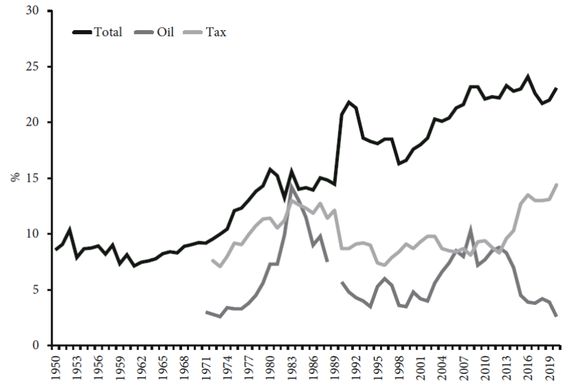
Note: Series are not comparable from 1970 to 1989 due to their different sources.
Source: Author’s elaboration using data from Mauro et al. (2013), Bazdresch and Levy (1991), the World Development Indicators database of the World Bank, and Estadísticas Oportunas de Finanzas Públicas database of the SHCP.
Figure 2 Total, oil, and tax revenues as a percentage of GDP, 1950-2020
Table 1 Tax revenue as a percentage of GDP
| Country | 2018 | Country | 2018 |
|---|---|---|---|
| Brazil | 33.1 | Colombia | 19.3 |
| Belize | 29.7 | Peru | 16.4 |
| Argentina | 28.8 | Mexico | 16.2 |
| Jamaica | 27.8 | Paraguay | 14.0 |
| Costa Rica | 24.0 | Dominican Republic | 13.2 |
| Ecuador | 20.6 | Guatemala | 12.1 |
Source: Author’s elaboration using data from the Global Revenue Statistics Database of the Organisation for Economic Co-operation and Development (OECD).
tr has not been as significant as in other economies with an income level similar to Mexico and, given the equilibrated/surplus primary balance rule followed by the Mexican government from 1950 to 2020, it has resulted in a small size of government intervention. As shown in Table 2, even for different lags, it is accepted that total public expenditure as a percentage of GDP (pe) does not Granger cause pr, while it is rejected that pr does not Granger cause pe.
Table 2 Granger causality tests between total public revenues and expenditures, 1950-2020
| Null hypothesis | 1 lag | 2 lags | 3 lags | 4 lags |
|---|---|---|---|---|
| pe does not Granger cause pr | 0.97 | 1.12 | 0.73 | 1.14 |
| pr does not Granger cause pe | 4.58** | 4.45** | 4.41* | 2.89** |
Notes: * and ** are statistically significant at the 1% and 5% levels, respectively. All series are in natural log terms. The reported value is the F-Statistic.
Source: Author’s elaboration using data from Mauro et al. (2013) and Estadísticas Oportunas de Finanzas Públicas database of the SHCP.
As a more rigorous proof of the causal relationship from pr to pe, we estimate the following long-run equation:
where β i are the parameters to be estimated, T is the time index and upe is an error term. Before estimating the long-run equation [19], we show in Table 3 the unit root test for the time series used. As it can be seen, pe is a stationary series while pr and pr2 are integrated of order 1. To estimate the long-run equation [19], we use the bound test approach (BTA) cointegration methodology (see Pesaran, Shin, and Smith, 2001)5. The results of our estimation are shown in Table 4.
Table 3 Unit root test for total public expenditures and revenues as a percentage of GDP, 1950-2020
| Variable | peT | prT | d(prT) | pr2T | d(pr2T) |
|---|---|---|---|---|---|
| Augmented Dickey-Fuller (ADF) test | -3.36*** | -2.83 | -10.75* | -3.00 | -9.68* |
| Phillips-Perron (PP) test | -3.37*** | -2.66 | -10.76* | -3.00 | -9.69* |
Notes: * and *** are statistically significant at the 1% and 10% levels, respectively. d(·) stands for the first difference operator. All series are in natural log terms. Level tests assume intercept and trend; first differences tests for pr assume intercept but no trend, and first differences tests for pr2 assume no intercept and no trend. The numbers of lags used for the ADF tests were chosen according to the Schwarz information criterion, whereas the numbers of Bandwidth used for the PP tests were chosen according to the Newey-West criterion.
Source: Author’s elaboration using data from Mauro et al. (2013) and Estadísticas Oportunas de Finanzas Públicas database of the SHCP.
Table 4 Estimation of the total public expenditures as a percentage of GDP, 1950-2020
|
Dependent variable:
pet Long-run relationship | |
|---|---|
| Constant | 4.43* |
| (0.95) | |
| prT | -2.43* |
| (0.75) | |
| pr2T | 0.64* |
| (0.14) | |
| D8389T | -0.72* |
| (0.06) | |
| Model type | Restricted constant, no trend |
| Autoregressive Distributed Lag (ARDL) model | (3, 3, 3, 0) |
| F-Bounds test | |
| F-Statistic | 10.30* |
| Adjustment coefficient | |
| upeT-1 | -0.52* |
| Jarque-Bera test | 0.40 |
| LM test (F-statistic, 1 lag) | 0.70 |
| White test (F-statistic)a/ | 1.61 |
| Ramsey Reset test (t-statistic, 1 fitted term) | 0.33 |
Notes: * is statistically significant at the 1% level (standard errors in parenthesis). a/ White test does not include cross terms. We use a dummy variable to capture a structural break; D8389 stands for a dummy variable with value equal to 1 from 1983 to 1989 and 0 otherwise. ARDL model indicates the number of lags of the dependent and independent variables. A complete report of the estimation, including the fixed regressors, is available on request from the author.
Source: Author’s elaboration using data from Mauro et al. (2013) and Estadísticas Oportunas de Finanzas Públicas database of the SHCP.
According to our results, pe behaves as a quadratic function of pr. As can be seen in Figure 3, our estimation is consistent with the idea of pr acting as a pe constraint. Except for the 1983-1989 subperiod in which pe was strongly decreased to cover debt and debt services, the estimated long-run equation generally indicates a lower value, although not significantly different, of pe with respect to pr.

Source: Author’s elaboration based on the long-run estimated equation reported in Table 4.
Figure 3 Long-run relationship between total public revenues and expenditures as a percentage of GDP, 1950-2020
As it is known, public expenditure can be registered in two accounts, the public balance and the national account. Given that the issues registered in both accounts are not the same, it is worth noting that there is a strong relationship between the total public expenditure registered in the public balance (PE) and the total public expenditure recorded in the national accounts (GG). From 1950 to 1960, the correlation coefficient between pe and GG as a percentage of GDP (gg) was equal to 0.66; from 1961 to 1989, it was equal to 0.85, and from 1990 to 2020, it was equal to 0.88 (see Figure 4). Therefore, pr is not only a constraint for pe but so is also for gg.

Source: Author’s elaboration using data from Mauro et al. (2013), Estadísticas Oportunas de Finanzas Públicas database of the SHCP and the World Development Indicators database of the World Bank.
Figure 4 Total public expenditure recorded in the public balance and the national accounts as a percentage of GDP, 1950-2020
According to Figure 5, from 1950 to 1981 gg doubled, from 11.4% to 22.9%. Then, from 1982 to 2020, it exhibited a cyclical behavior with the lowest value in 1996 (10.5%) and the highest value in 2009 (17.9%). Thus, from 1982 to 1996, the extent of government intervention in the economy was completely reversed. Furthermore, although its importance began to increase again in 1997, the 2009 crisis truncated the process without reaching the 1981 level. However, there was not only a reduction in the size of government intervention from 1982 on, but there was also a structural change in the composition of GG. As shown in Figure 6, from 1950 to 1981 the annual averages of PC and I pu as a GG percentage were equal to 48.8% and 51.2%, respectively, while from 1982 to 2020, they were equal to 70.8% and 29.2%, respectively.

Source: Author’s elaboration using data from the CEPALSTAT database of the Economic Commission for Latin America and the Caribbean (ECLAC), the World Development Indicators of the World Bank, and Estadísticas Oportunas de Finanzas Públicas database of the SHCP.
Figure 5 Total public expenditure registered in the national accounts as a percentage of GDP, 1950-2020

Source: Author’s elaboration using data from the CEPALSTAT database of ECLAC, the World Development Indicators database of the World Bank, Estadísticas Oportunas de Finanzas Públicas database of the SHCP and Hofman (2000).
Figure 6 Public consumption (PC) and public investment (Ipu) as a percentage of total public expenditure (GG), 1950-2020
It is worth noting that Ipu , as a GG percentage, exhibited a slightly negative trend from 1950 to 1981, and it was accentuated from 1982 to 2020. In such a way, Ipu , as a GG percentage, decreased from 58.8% in 1950 to 17% in 2020.
The substantial reduction of I pu has negatively affected the growth rate of the economy (g) (see Figure 7). It is also worth noting that Ip did not decrease with the fall of Ipu, but it increased more than the absolute decrease of Ipu, in such a way that the annual average of the total investment as a percentage of GDP was higher from 1982 to 2020 (20.2%) than from 1951 to 1981 (18.1%). However, beyond debating the existence or non-existence of a crowding-out effect, the productivity of investment was lower with the restructuring of I in favor of Ip6.

Source: Author’s elaboration using data from Hofman (2000), the World Development Indicators database of the World Bank, the CEPALSTAT database of ECLAC, and Banco de Información Económica database of the Instituto Nacional de Estadística y Geografía (INEGI).
Figure 7 Public investment as a percentage of GDP and annual growth rate, 1951-2020
To evaluate the importance of Ipu for g, we estimate the following long-run equation:
where θi are the parameters to be estimated, Z is an independent variable [we use three different candidates: Ipu and Ip as a percentage of GDP (ipu and ip respectively) and the exports growth rate (x)], and uZ is an error term. Before estimating the long-run equation [20], Table 5 shows the unit root test for the time series used. As shown, all the variables are stationary. To estimate the long-run equation [20], we use the BTA cointegration methodology7. The results of our estimation are shown in Table 6.
Table 5 Unit root test for the output and exports annual growth rates, and public and private investment as a percentage of GDP, 1950-2020
| Variable | gT | ipuT | ipT | xT |
|---|---|---|---|---|
| ADF test | -4.72* | -1.32 | -3.73** | -5.80* |
| PP test | -4.69* | -1.51 | -3.81** | -5.72* |
| ADFBPT test | -4.85** | |||
| (1990) |
Notes: * and ** are statistically significant at the 1% and 5% levels, respectively. ADFBPT is the Augmented Dickey-Fuller unit root test considering one breakpoint, break year between parentheses. Level tests assume intercept and no trend. The number of lags used for the ADF tests were chosen according to the Schwarz information criterion, whereas the number of Bandwidth used for the PP tests were chosen according to the Newey-West criterion.
Source: Author’s elaboration using data from Hofman (2000), the World Development Indicators database of the World Bank, the CEPALSTAT database of ECLAC, and Banco de Información Económica database of the INEGI.
Table 6 Estimation of the annual growth rate, 1950-2020
|
Dependent variable:
gT
Long-run relationship | |||
|---|---|---|---|
| Period | 1950-2020 | 1950-2020 | 1961-2020 |
| Constant | 11.60* | ||
| (1.49) | |||
| ipuT | 0.54* | ||
| (0.18) | |||
| iPT | -0.52* | ||
| (0.11) | |||
| xT | 0.57* | ||
| (0.13) | |||
| Model type | Unrestricted constant, no trend | Restricted constant, no trend | Unrestricted constant, no trend |
| ARDL model | (1, 1) | (1, 0) | (4, 4) |
| F-Bounds test | |||
| F-Statistic | 29.31* | 26.35* | 11.77* |
| t-Bounds test | |||
| t-Statistic | -7.60* | -4.25* | |
| Adjustment coefficient | |||
| uZT-1 | -0.85* | -0.84* | -0.53* |
| Jarque-Bera test | 4.48 | 2.53 | 2.45 |
| LM test (F-statistic, 1 lag) | 1.31 | 0.14 | 1.01 |
| White test (F-statistic) | 0.69 | 0.35 | 0.29 a/ |
| Ramsey Reset test (t-statistic, 1 fitted term) | 0.15 | 0.09 | 1.81*** |
Notes: * and *** are statistically significant at the 1% and 10% levels, respectively (standard errors in parenthesis). a/ White test does not include cross terms. ARDL model indicates the number of lags of the dependent and independent variables. A complete report of the estimation, including the fixed regressors, is available on request from the author.
Source: Author’s elaboration using data from Hofman (2000), the World Development Indicators database of the World Bank, the CEPALSTAT database of ECLAC, and Banco de Información Económica database of the INEGI.
As can be seen in Table 6, for the three cases the estimated parameter is statistically significant. However, in the case of ip the estimated relationship is negative. On the other hand, although the estimated relationships are positive for ipu and x, according to the Ramsey Rest test, there is a specification problem in the equation including x. Moreover, both the F-Statistic and the t-Statistic are lower in absolute value for the estimation including x than for that including ipu . Furthermore, the error correction term is higher for the estimation including ipu than for that including x.
As for the negative effect of ip on g, it could be a result from the structural change experienced by the Mexican economy after the economic liberalization process. With the General Agreement on Tariffs and Trade, and especially with the North American Free Trade Agreement (NAFTA), United States-Mexico-Canada agreement (USMCA) nowadays, there was a stimulus for private investment in a context of a new international division of labor in which developing economies are inserted in low added value activities of the global value chains. This phenomenon could be an explanation for the negative estimated relationship between ip and g. Before the 1982 debt crisis ipu was significant and it was related to an industrialization process in which the Mexican economy was creating its domestic value chains (see Moreno-Brid and Ros, 2009). This could be an explanation for the positive stated relationship between ipu and g.
Moreover, as indicated above, the reduction of Ipu implies a negative effect on NX, causing the balance of payments constraint to become stronger. To show the positive effect of Ipu on NX, we estimate the following long-run equation:
where αi are the parameters to be estimated, nx and pc are NX and PC as a percentage of GDP, respectively, and unx is an error term. Before estimating the long-run equation [21], Table 7 shows the unit root test for the time series used. As shown, all the series are stationary. Finally, using the BTA cointegration methodology8, our estimation results of the long-run equation [21] are shown in Table 8.
Table 7 Unit root test for the annual trade balance and public consumption as a percentage of GDP, 1950-2020
Notes: * and *** are statistically significant at the 1% and 5% levels, respectively. d(·) stands for the first difference operator. Level tests for nx assume intercept and no trend, while for pc assume intercept and trend; first differences tests for pc assume intercept but no trend. The numbers of lags used for the ADF tests were chosen according to the Schwarz information criterion, whereas the number of Bandwidth used for the PP tests were chosen according to the Newey-West criterion.
Source: Author’s elaboration using data from Hofman (2000), the World Development Indicators database of the World Bank, the CEPALSTAT database of ECLAC, and Banco de Información Económica database of the INEGI.
Table 8 Estimation of the annual trade balance as a percentage of GDP
|
Dependent variable:
nxT
Long-run relationship | ||
|---|---|---|
| Period | 1961-2020 | 1951-2020 |
| Constant | -2.79*** | |
| (1.49) | ||
| gT | -0.67* | -0.77* |
| (0.14) | (0.23) | |
| ipuT | 0.80** | 0.83** |
| (0.36) | (0.32) | |
| pcT | -0.36 | |
| (0.35) | ||
| ipT | 0.14 | |
| (0.30) | ||
| Model type | Unrestricted constant, no trend | Restricted constant, no trend |
| ARDL model | (2, 0, 1, 3, 0) | (3, 0, 1) |
| F-Bounds test | ||
| F-Statistic | 18.22* | 7.26* |
| t-Bounds test | ||
| t-Statistic | -5.41* | |
| Adjustment coefficient | ||
| unxT-1 | -0.39* | -0.21* |
| t-Bounds test | ||
| t-Statistic | -9.89* | |
| Jarque-Bera test | 0.22 | 3.35 |
| LM test (F-statistic, 1 lag) | 1.24 | 0.11 |
| White test (F-statistic) | 1.58 a/ | 1.12 |
| Ramsey Reset test (t-statistic, 1 fitted term) | 0.63 | 1.43 |
Notes: *, ** and *** are statistically significant at the 1%, 5%, and 10% levels, respectively (standard errors in parenthesis). a/ White test does not include cross terms. ARDL model indicates the number of lags of the dependent and independent variables. A complete report of the estimation, including the fixed regressors, is available on request from the author.
Source: Author’s elaboration using data from Hofman (2000), the World Development Indicators database of the World Bank, the CEPALSTAT database of ECLAC, and Banco de Información Económica database of the INEGI.
As shown in Table 8, the estimated parameters corresponding to pc and ip have the expected signs, but they are not significant; on the other hand, the estimated parameters corresponding to g and ipu have the expected sign, and they are statistically significant. Moreover, even if we remove pc and ip from the estimation, the estimated parameters corresponding to g and ipu are not very different, especially for ipu . Therefore, the reduction of Ipu has involved a more restricted balance of payments constraint.
4. Conclusion
Although Keynes’s theory has been identified with fiscal deficit budgets to compensate insufficient aggregate demand during recessive periods, in fact he did not propose the use of public consumption, or direct income tax for that matter, to tame the economic cycles beyond the working of the automatic stabilizers.
According to Keynes (1980b), the true problem is that the volume of private investment tends to be less than enough to generate a full-employment level of output. He maintained that it is necessary to socialize the investment function through an ambitious public investment program to keep the output level at the equilibrium position and reduce the fiscal deficit budget required during recessive periods. Keynes argued that fiscal policy should not be used to bridge aggregate demand gaps, but to prevent the latter.
As shown, by implementing a tax rate to obtain financial resources the government can increase the level of output, but, at the same time, disposable income is reduced given the increase of the demand for imports and the consequent rise of external savings. On the other hand, if the government implements a public investment program, it can reduce the demand for imports and external savings, allowing for an increase in disposable income. In fact, if the marginal negative effect of investment on the demand for imports is higher than the marginal positive effect of income, then disposable income will be higher if there is government intervention than if there is not.
As argued above, after the 1982 debt crisis the Mexican economy followed a balanced fiscal budget rule, but public investment lost its importance, giving room to a higher prominence of public consumption.
The reduction in public investment negatively affected the annual output growth rate, while private investment increases did not improve economic activity. In fact, it seems that investment productivity decreased drastically with the share of private investment increasing its participation in total investment. Moreover, the substantial public investment reduction has negatively affected the trade balance as well, tightening the external constraint on growth, a stylized fact consistent with the slow growth regime of the Mexican economy since the 1982 debt crisis.
As mentioned before, Keynes did not just consider direct income tax as a source of public revenues; however, as it is known, tax revenues are, in general, the primary source of the government finance. So, Mexico’s tax effort must increase to raise the necessary resources for implementing an ambitious public investment program aimed at taming business cycle volatility and improving the growth rate of the economy, not just directly but also indirectly through the relaxation of the external constraint. Therefore, a progressive tax reform could do the twofold job of raising public revenues and stimulating aggregate demand while modifying income distribution in favor of the poorest population with the highest marginal propensity to consume.

