


 nueva página del texto (beta)
 Inglés (pdf)
 Artículo en XML
 Referencias del artículo
 Enviar artículo por email
 Citado por SciELO
  Similares en
SciELO
Similares en
SciELO 
 Permalink
1. Introduction
Since the early 1970s, Chile’s economic policy has been guided by free market ideology, and up until the unexpected eruption of social protests and unrest in the last quarter of 2019, the Chilean model was considered a success story. The main building blocks of the Chilean economic model are well known. These include the extended privatization of the productive apparatus (with a few exceptions including mining, energy, and basic services); the liberalization of finance and trade; political and operational independence of the central bank to achieve price stability; and the use of implicit and explicit fiscal rules to discipline public spending and contribute to ensure an adequate credit rating for the economy as a whole.
The role of the government in Chile has been limited to maintaining a minimum social safety net and to correct for market imperfections. The success of the Chilean model has been predicated on the achievement of nominal stability (price stability accompanied with low fiscal deficits and public debt), low levels of unemployment (even though under employment and informality remained high), decreasing poverty rates, and increasing per capita income levels.
From the mid-1980s to the end of the 1990s decade, Chile doubled its Gross Domestic Product (GDP) per capita. Later Chile became the second Latin American country after Mexico (1994) to be accepted as a member of the Organisation for Economic Co-operation and Development (OECD), and in 2014, Chile was classified as a high-income country2.
Despite their merits, these achievements hardly provide a complete and accurate picture of the Chilean economic model. A closer analysis shows that it is built on weak foundations that undermine its portrayal as a free market/neoliberal success.
Since the middle of the 1990s Chile exhibits a declining trend in the rate of growth of GDP. At the same time, the functional distribution of income clearly displays an increase in the profit over the wage share. Declining growth trend and a rising profits share have been accompanied by increasing private debt levels including those of households and of the corporate sector. Currently, Chile is one of the most indebted countries in the developing world.
This paper argues that lower trend growth with increased inequality and rising indebtedness constitute a perfect mix for a context of financial fragility. It is divided into four sections. The second section analyses and explains the decline in the growth trend of the Chilean economy, the existing inequality in terms of the functional distribution of income. and debt accumulation. The third section focusses on the notion of financial fragility. The fourth and fifth sections analyse the existence of financial fragility for the corporate and household sectors. The last section concludes.
2. A characterization of the Chilean economic model
2.1. The decline in the trend growth rate
An in-depth analysis of the different dimensions of the country’s economic development and evolution over time indicates that since the middle 1990s, the Chilean economy exhibits a persistent decline in its long-term growth rate. The trend rate of growth of GDP declined on average from 6.6% in the 1990s, to 4.4% in the 2000s to a 2.9% in the period 2010-2019. In the past two years the rate of growth of GDP has settled at 1.5% (see Table 1).
Table 1 Selected economic and social indicators, 1980-2019 (averages)
| 1980s | 1990s | 2000s | 2010-2019 | |
|---|---|---|---|---|
| Growth and income | ||||
| GDP growth trend (percentages) a/ | 3.4 | 6.6 | 4.4 | 2.9 |
| GDP per capita a/ | 5,034 | 7,739 | 10,976 | 14,377 |
| Composition of GDP by sector of economic activity | ||||
| Natural resources (per cent of GDP) | 15 | 23.9 | 23.4 | 17.5 |
| Mining (per cent of GDP) | 9.0 | 20.2 | 19.7 | 14.0 |
| Manufacturing (per cent of GDP) | 20.8 | 14.7 | 12.3 | 10.3 |
| Finance (per cent of GDP) | 9.1 | 14.9 | 17.8 | 20.5 |
| Investment (per cent of GDP) | 18.0 | 24.8 | 21.6 | 23.0 |
| Productivity b/ | ||||
| Productivity growth | -0.01 | 4.6 | 1.8 | 0.8 |
| Relative productivity | - | 37.7 | 41.5 | 41.2 |
| Research and development expenditure (per cent of GDP) c/ | - | - | - | 0.36 |
| Technological intensity d/ | ||||
| Economic Complexity Index (ECI) | 0.04 | 0.05 | -0.11 | -0.02 |
| Engineering Intensity Index (EII) | 18.1 | 20.4 | 24.8 | 31.2 |
| Poverty and inequality e/ | ||||
| Poverty | 45.1 | 27.4 | 31.5 | 14.2 |
| Gini | 56.2 | 55.8 | 49.7 | 45.2 |
Notes: a/ The GDP growth trend was computed using a Hendrick-Prescott filter. GDP and its composition by sector expressed in constant 2010 US$ dollars. b/ Productivity refers to labour productivity. Relative productivity refers to Chile’s labour productivity relative to that of the United States. c/ Corresponds to the average for the period 2007-2017.d/ EII is the ratio between the share of high technology manufacturing exports in Chile relative to the share of high technology exports in the United States. Higher values of both indices imply greater technological intensity. For EII the data reported for the 2000s decade correspond to the 2007-2009 average. e/ Poverty headcount ratio at national poverty lines (per cent of population). For Gini the data reported for the 1980s decade correspond to the point value for 1987.
Source: Banco Central de Chile (2020b), World Bank (2020), OECD (2020a) and ECLAC (2020).
This downward trend in GDP growth can be explained by a deteriorating performance in the main determinants of long-term growth, including investment and productivity. The evolution of investment and of its most important component, machinery and equipment (the component with the highest technology content, which can contribute most to economic growth), shows a loss of dynamism since the 1990s. Total investment averaged 24.8%, 21.6%, and 23.0% of GDP for the 1990s, 2000s, and for the period 2010-2019, respectively. Machinery and equipment follow a similar trend with 12.4% and 10.8% of GDP for the 1990s and 2000s, respectively. In line with these observations, factor productivity expanded at a rate of 4.6%, 1.8% and 0.8% for the 1990s, 2000s and 2010-2019, respectively
The weak productivity performance is exemplified in the decline and low values of the economic complexity and engineering intensity indices. The former reflects information regarding the diversity and sophistication of a country’s exports. The latter captures a country’s share of high technology manufacturing exports relative to that of the United States. In the case of the engineering intensity index, the value obtained by Chile for the 2000s means that its proportion of high technology manufacturing exports relative to the total represents 24.8% of that of the United States.
2.2. High inequality
The decline in the growth trend has been accompanied by high levels of inequality even though Chile has managed to significantly reduce poverty3. Chile exhibits one of the highest levels of inequality in the OECD. Since the 1990s, the Gini coefficient for Chile remained above 50 until the middle of the 2000s, dropping slightly to reach 46.6 in 2017, surpassing the average registered for Latin America and middle-income countries in general. Chile currently holds the 26th place in income inequality in the world. Moreover, when capital gains (or retained profits and evasion corrections) are included in the measurement of inequality, the value of Gini coefficient is above 60 and the top 1% of households receive over 30% of total income.
Inequality is not only prevalent in terms of personal income but is also visible when measured in terms of the functional distribution of income. Figure 1 above shows the distribution of income between wages and profits for the period 1985-2018. As the figure clearly shows the profit share has always outpaced the wage share. Moreover, the profit share increased significantly since the beginning of the 2000s decade rising from 45% in 1999 to 54% in 2019. For the same period, the wage share showed only a slight increase (40% to 43% for the same years).
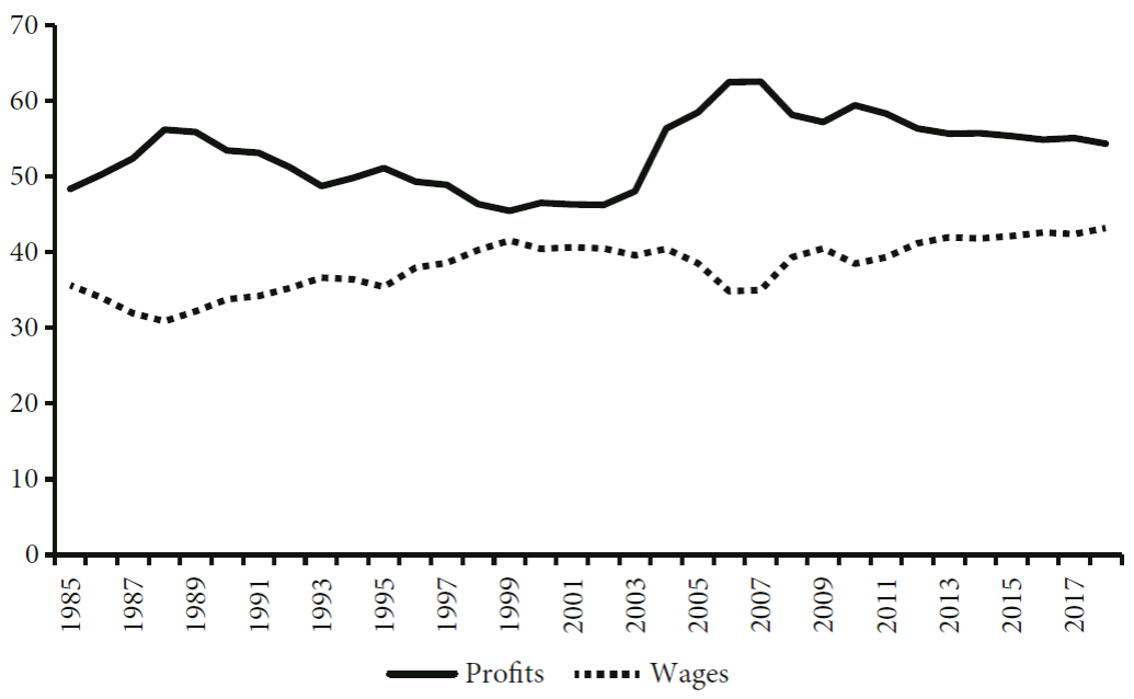
Source: Banco Central de Chile (2020b).
Figure 1 Functional distribution of income, 1985-2018 (percentage of total income)
2.3. Increasing debt accumulation
A lower trend growth rate and greater inequality have created the conditions for debt accumulation. Figure 2 shows the evolution of total debt by economic sector (households, non-financial corporate sector, and the government) for the period 2002-2020. Four stylized facts characterize the evolution and composition of debt. First, since 2007 no sector has been spared from increasing indebtedness. Debt has steadily increased for households, non-financial corporate sector, the financial sector, and the general government.

Note: The data corresponding to non-continuous lines are displayed on the right axis.
Source: Banco Central de Chile (2020a and 2020b).
Figure 2 Total debt by economic sector as a percentage of GDP, 2002-2020
Second, debt is rising faster than GDP (income). In 2007, the aggregate debt to GDP ratio stood at 111.5% rising to 203% in 2020 (340% of GDP if the financial sector is included). As things stand, Chile is one of the most indebted emerging market economies in the world. Third, the accumulation of debt is concentrated in the private sector. The bulk of the stock of debt is held by the financial sector and non-financial corporate sector. The debt stock of both sectors represented 141% and 120% of GDP for March 2020 accounting for 40.9% and 34.9% of the total, respectively. If the financial sector is excluded the debt of the non-financial corporate sector represented 59% of total debt. Also, the sector accounts for more than 60% of total external debt. The debt of the household sector represented 52% of the total in the first quarter of 2020. The government is the sector with the lowest debt level (33% of GDP for March 2020 accounting for only 9.6% of the total).
Fourth, external debt has also been on the rise (30.7% of GDP in December 2007 and 82.9% March 2020) [see Figure 3] and the non-financial corporate sector accounts for 60% of total external debt. This has major implications not only for overall debt sustainability and for investment and growth. Increased external debt takes on a particular importance since the sector is characterized by currency mismatch4. The depreciation of local currencies can affect firms’ financial situation. Depreciation not only raises debt service costs, and thus expenditures, but also swells liabilities by increasing the local-currency value of outstanding debt. If the collateral for the debt is likewise denominated in local currency, depreciation will also cause this asset to lose value. This can give rise to a mismatch such that the firm must purchase currency to balance its accounts. Depending on its size and importance in the market and the number of firms behaving in this way, currency purchases can create further pressure for devaluation of the nominal exchange rate, ultimately increasing the external debt of the firms operating in the non-tradable goods sector. In turn, the negative effect of exchange rate depreciation on firms’ balance sheets can inhibit investment (Caballero, 2020)5.
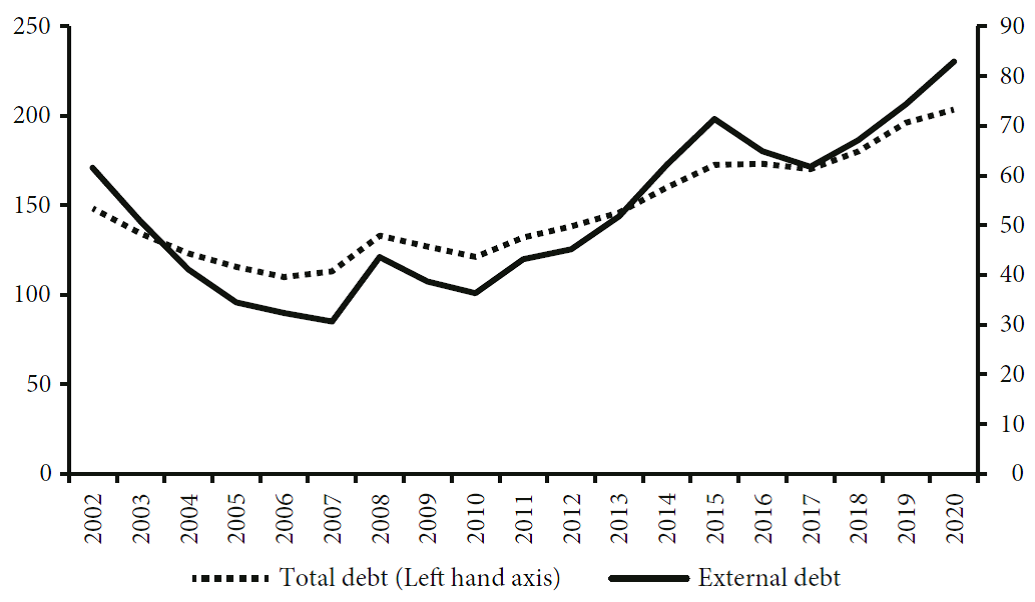
Source: Banco Central de Chile (2020a and 2020b).
Figure 3 Evolution of total and external debt, 2002-2020 (percentage of GDP)
3. A conceptual analysis of financial fragility
A macroeconomic context characterized by a combination of low trend growth, high inequality and increasing debt to GDP ratios for the economy at the aggregate level can easily evolve into one characterized by financial fragility. Financial fragility refers to a situation where growing indebtedness generates increasing debt payments commitments that will eventually exceed income cash flows.
Financial fragility is the result of the workings of an economy in which lending and borrowing take place based on a decrease in the size of the margins of safety. The margins of safety are provided by liquidity (cash receipts and liquid assets) and allow for ‘error and variance’ (Minsky, 1975, p. 162). As explained by Minsky (1986, pp. 79-80):
The margins of safety can be identified by the payment commitments on liabilities relative to cash receipts, the net worth or equity relative to indebtedness (…), and the ratio of liabilities to cash and liquid assets, that is the ratio of payment commitments to assets that are superfluous to operations. The size of the margins of safety determines whether a financial structure is fragile or robust and in turn reflects the ability of units to absorb shortfalls of cash receipts without triggering a debt deflation.
As the margins of safety decrease economic agents become more dependent on income flows for debt payments and the ‘normal functioning of financial markets to refinance positions in long-term assets.’ As a result, any disruptions in income or in financial markets, can lead economic agents to experience difficulties in paying their debt (debt service and or principal) leading to liquidity constraints and outright insolvency. The size and strength of margins of safety of the different sectors in an economy, as well as the likelihood that an initial disturbance is amplified, determines the robustness or fragility of an economy (Minsky, 1986, p. 209)6.
The size and strength of the margins of safety are ‘safest’ when economic agents can repay their debt (interest and principal) commitments with future cash flows. The size and strength of the margins of safety are the least safe when economic agents rely on the expectation of an appreciation of the underlying asset(s) which sustains their debt or of a favourable change in the underlying economic conditions (say an appreciation of the exchange rate when debt is denominated in foreign currency) to cover their liabilities (interest and principal). In between both extremes is the case where economic agents expect future cash flows to cover interest payments but not the principal.
The more dominant are the Ponzi and speculative regimes over hedge financing at the agent, sector, and economy wide levels, the greater is the thrust towards financial fragility and instability. Hedge financing regimes depend only on expected income flows, that is, on the state of the labour and goods and services markets, and hence on the state of the economy in the aggregate. Speculative and Ponzi finance depend in addition on financial market conditions. A speculative regime implies the possibility of rolling over debt to repay the principal. A Ponzi regime cannot last for very long, and thus implies the possibility of increasing debt to pay for debt, selling assets or reconfiguring portfolios to meet payment commitments.
The prevalence of hedge, speculative or Ponzi regimes is generally associated with the type of debt of economic agents. When debt is not tied to the expected income streams of some underlying asset, then that debt is considered as part of hedge financing. Consumer household debt is generally considered hedge financing. However, depending on its characteristics Household mortgage debt can be categorized as speculative and/or Ponzi finance. Also, consumer and household debt can amplify business cycle fluctuations. As explained by Minsky, (Minsky, 1982, p. 30):
The typical financing relation for consumer and housing debt can amplify but it cannot initiate a downturn in income (…). However, a part of household financing is often Ponzi; this is the financing of holdings of securities and some type of collectible assets. A typical example is the financing of ownership of common stocks or other financial instruments by debts.
In this regard household finance can be “destabilizing if there is a significant portion of Ponzi finance in the holding of financial and other assets.” (Ibid., p. 31).
However, Minsky made clear that while the financing of consumption is mainly hedge finance, a fall in wages can transform hedge into Ponzi finance (Ibid., p. 32). Also, reliance on consumer credit can also be a source of financial fragility (Lavoie, 2014, p. 254). An extra complication to which we make reference in footnote 12 below is that household surveys do not capture the debt information (especially that pertaining to assets) and in fact may understate the extent to which households are in a fragile financial position.
The financing regimes of non-financial corporate and financial sectors are easily classifiable under speculative or Ponzi categories as their debt depends on the underlying value of an asset or a given set of assets. The following two sections of the paper provide a financial analysis -along Minskyan lines- of financial fragility in the corporate and household sectors in Chile.
4. Financial fragility in the non-financial corporate sector
4.1. Methodology and data set
The financial fragility of the non-financial corporate sector in Chile is analyzed for the period 2010-2019, on the basis of the existing literature that establishes measurable criteria and a threshold for distinguishing between the hedge, speculative, and Ponzi categories. More specifically, the criteria and thresholds used in the analysis follow the definitions by Mulligan (2013) and by Torres Filho, Marins, and Miaguti (2017).
The criterion used by Mulligan (2013) is the interest coverage ratio (IC). The criterion is defined as:
Mulligan establishes the following thresholds:
The criterion proposed by Torres Filho, Marins, and Miaguti (2017) is the financial fragility index (FFI) and it is defined as:
Where FO = financial obligations, STD = stock of short - term debt, EBITDA = earnings before interest, taxes, depreciation and amortization.
On this basis the thresholds for hedge, speculative, and Ponzi financial positions are established as follows:
The data set of firms used in the analyses was obtained from the Commission for the Financial Market of Chile (CMF, Comisión para el Mercado Financiero). The CMF publishes information of Financial Statements of Chilean firms following the norms of the International Financial Reporting of Securities Issuers (IFRS) and other entities operating in the Chilean market.
This was complemented with data obtained from the Chilean Internal Revenue Service (SII, Servicio de Impuestos Internos) that provides information for the payroll of taxpayers and legal entities listed as companies by the SII7. The data includes, among other variables, sales, number of dependant workers, regional and urban/rural location, and main economic activity.
The number of firms for which the criteria and thresholds defined by Mulligan (2013) and Torres Filho, Marins, and Miaguti (2017) were computed averages 562 for the entire period 2010-2019 with a standard deviation of 46 (the sample differs from year to year as shown in Table 2).
Table 2 Number of firms included in the analysis by year
| Year | Number of firms |
|---|---|
| 2010 | 425 |
| 2011 | 588 |
| 2012 | 575 |
| 2013 | 589 |
| 2014 | 589 |
| 2015 | 582 |
| 2016 | 567 |
| 2017 | 563 |
| 2018 | 567 |
| 2019 | 572 |
| Average | 562 |
| Standard deviation | 46 |
Source: CMF (2020).
4.2. Financial fragility in the non-financial corporate sector: Results
Table 3 presents the results for all firms in the aggregate and Figure 4 by firm size. Table 3 shows an increase in the percentage of firms that are financially fragile. Between 2011 and 2019 the percentage of firms considered to be fragile (belonging to a speculative or Ponzi financing regime) increased according to the two criteria considered. According to the IC criteria, these increased from 38% to 41% between 2011 and 2019. According to the FFI criteria, the proportion of firms that are on a fragile financial scheme increased from 16.1% to 21.6% between 2011 and 2019. Also, Table 3 reveals that the percentage of Ponzi firms increased according to the FFI criterion from 13.7% to 19.2% between 2010 and 2019, according to the FFI criterion.
Table 3 Proportion of total companies reporting balance sheets and income statement by year characterized by a hedge, speculative or Ponzi position, 2010-2019
| IC | FFI | |||||||
|---|---|---|---|---|---|---|---|---|
| Ponzi | Speculative | Fragile a/ | Hedge | Ponzi | Speculative | Fragile a/ | Hedge | |
| 2010 | 22.7 | 29.4 | 52.1 | 47.9 | 13.7 | 1.9 | 15.6 | 84.4 |
| 2011 | 17.3 | 20.7 | 38.0 | 62.0 | 14.3 | 1.8 | 16.1 | 83.9 |
| 2012 | 19.1 | 26.2 | 45.2 | 54.8 | 15.0 | 2.8 | 17.8 | 82.2 |
| 2013 | 15.6 | 25.1 | 40.7 | 59.3 | 17.3 | 1.5 | 18.9 | 81.2 |
| 2014 | 15.0 | 24.5 | 39.5 | 60.5 | 18.8 | 1.2 | 20.1 | 79.9 |
| 2015 | 17.3 | 22.8 | 40.1 | 59.9 | 17.9 | 2.5 | 20.4 | 79.6 |
| 2016 | 18.0 | 24.2 | 42.1 | 57.9 | 18.6 | 2.6 | 21.2 | 78.9 |
| 2017 | 18.0 | 22.4 | 40.4 | 59.6 | 18.5 | 1.7 | 20.2 | 79.8 |
| 2018 | 14.2 | 25.0 | 39.2 | 60.8 | 17.5 | 2.2 | 19.8 | 80.3 |
| 2019 | 15.6 | 25.4 | 41.0 | 59.0 | 19.2 | 2.4 | 21.6 | 78.4 |
Note: a/ The fragile column shows the sum of the Ponzi and speculative position.
Source: CMF (2020) and SII (2020).
Also, we computed the number of dependent workers per firm for each year according to the different criteria defined above. For the period 2010-2018, the average number of dependent workers that were working in firms with fragile positions were 84,483 and 17,794 according to the IC and FFI criteria, respectively. In accordance with these criteria, the above represents the 36.4% and 7.6%8 of total workers for the firms that we could effectively calculate the indices. This gives an idea on how many workers could have been affected, and therefore be potentially unemployed, because of the social outbreak of the last quarter of 2019 and the current pandemic that we are facing9.
As expected, the subdivision by firm size shows that micro, small and medium (MSMEs) firms tend to exhibit a higher propensity towards financial fragility than larger firms. For the period 2010-2018, the percentage of MSMEs that are financially fragile reached 29% and 49% on average compared to 17% and 41% for larger firms according to the FFI and IC criteria, respectively. Nonetheless, the prevalence of financial fragility among larger firms can also be significant (41% of the total according to the IC criterion) [see Figure 4].
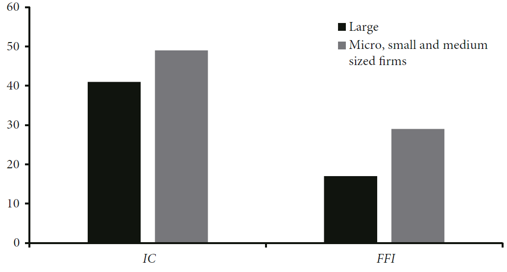
Note: The SII considers a firm as large if the annual sales are above 100,000.00 Unidades de Fomento in a year, and MSMEs otherwise. One Unidad de Fomento is equal to 28,686 Chilean Pesos (September 1st, 2020). The bilateral dollar-peso exchange rate is roughly 780 pesos for one dollar.
Source: CMF (2020) and SII (2020).
Figure 4 Percentage of large and micro, small and medium sized firms that are financially fragile using the IC and FFI criteria, 2010-2018 (averages)
One possible explanation for the higher proportion of smaller companies in fragile financial positions is the interest rate differential that both groups face. During 2013-2017 the average interest rate spread for large firms compared to micro, small and medium was 5.79%. Thus, the price of debt is much higher for smaller firms and can undermine their capacity to repay their obligations (OECD, 2020b).
To complete the analysis, we disaggregated the sample of companies according to the economic sector in which they perform in accordance with the International Standard Industrial Classification (ISIC). The evidence for 2018 shows a clear tendency for certain sectors to have a high proportion of speculative and Ponzi schemes. These include construction, financial and insurance activities as well as real estate activities (see Table 4 below).
Table 4 Proportion of companies reporting balance sheets and income statement by year with a fragile position (speculative or Ponzi) by sector of economic activity, 2018 (percentage of firms from the sector)
| Sector | FFI | IC |
|---|---|---|
| Construction | 30 | 72 |
| Information and Communications | 0 | 38 |
| Agriculture, Livestock, Forestry, and fisheries | 0 | 33 |
| Mining and Quarrying | 0 | 40 |
| Real Estate Activities | 55 | 42 |
| Financial and Insurance Activities | 28 | 36 |
| Transport and Storage | 18 | 59 |
| Wholesale and Retail Trade; Repair of Motor Vehicles | 23 | 8 |
| Electricity, Gas, Steam, and air Conditioning Supply | 19 | 41 |
| Manufacturing | 3 | 19 |
Source: CMF (2020) and SII (2020).
5. Financial fragility in the household sector
5.1. The indicators
Financial fragility of households is analyzed on the basis of four indicators. Three of these indicators are commonly used to measure the debt burden of households: The first indicator is the debt service-to-income ratio (DSIR), defined as the monthly debt payment relative to monthly net income. It reflects a household’s financial burden, its ability to pay off debt commitments without the need to resort to asset liquidation.
The second indicator corresponds to the debt-to-asset ratio
(DAR), which is defined as the value of the total debt with
respect to total assets. Unlike the DSIR, this indicator
reflects the possibility of repaying the debt with existing available assets.
The third indicator corresponds to the ratio between the total debt payment
(interest and principal) and monthly net income (DIR). This
reflects the burden of total debt relative to household income. It reflects the
number of months it would take for a household to pay its debt, assuming income
remains constant. The fourth indicator provides a measure of a Minskyan cushion
of safety for a household. This indicator is the financial margin of households
(FM) which is equal to net income from taxes
(I) minus debt payments (DP) and the cost
of living adjusted by the number of people in a household (
Formally,
We computed the first three debt indicators (DSIR, DAR and DIR) according to whether the type of debt held corresponded to mortgage or consumption debt (see Table 5). The results are presented by income deciles for both the mean and the median (see Table 7a). For the financial margin we present the results for total income, labor and pension income and labor income only.
Table 5 Indicators of financial fragility for the household sectors and their respective thresholds
| Indicator | Financial fragility threshold value |
|---|---|
| Debt service-to-income, DSIR Threshold Mean Median |
DSIR > 0.25 DSIR > 0.46 DSIR > 0.25 |
| Debt-to-asset ratio, DAR Threshold Mean Median |
DAR > 0.75 DAR > 1.61 DAR > 0.15 |
| Total debt payment (interest and principal) to income,
DIR
Threshold Mean Median |
DIR > 36 DIR > 12.5 DIR > 3.7 |
| Financial margin of households, FM
Threshold Mean Median |
FM < 0 FM < 651,411 FM < 338,250 |
Note: The threshold, mean and median for the financial margin of households is the average of the threshold, mean and median for the wage, pensions, and subsidies (Total income in Chilean pesos).
Source: Balestra and Tonkin (2018) and Banco Central de Chile (2018b).
The financial fragility of households was assessed on the basis of the mean, the median and threshold values for all indicators. By extension, the percentage of all households that find themselves above or below the mean, median or a given threshold was obtained. The values of the mean, median and thresholds for all the indicators referring to total debt are shown in Table 5 below.
The choice of thresholds values for the DSIR, DAR and DIR, follows the methodology of the Balestra and Tonkin (2018) and the Banco Central de Chile (2018a and 2018c). The rationale behind these criteria is based on the vulnerability of households when facing possible scenarios of income decline. Those households that use more than 25% of their monthly income for debt payments (DSIR) are in a situation of financial vulnerability, as well as those households whose debt value exceeds 75% of the value of their assets (DAR), or those who take more than 36 months to liquidate their full payment commitments (DIR) if they maintain their monthly income constant. In the case of the financial margin (FM) the threshold value was set at zero since a value less than zero means that households are not able to face their debt and consumer expenses with their available income sources.
The data used for the computation of the indicators was obtained from the latest Household Financial Survey 2017 (Encuesta Financiera de Hogares 2017) published by the Banco Central de Chile (2018b). This dataset is representative at the urban national level, with a total of 4,549 households interviewed. It comprises 128 variables including, among others, household and/or individual characterization, as well as asset values, debt, income, and financial products11.
5.2. An analysis of the empirical results12
Table 6a presents the percentage of households that are above the financial fragility threshold, and the mean and median of each of the indicators considered (DSIR, DAR, and DIR) by type of debt. Table 6b presents the results of households below the same indicators for FM by source of income. The results for total debt show that the percentage of households that are above the financial fragility threshold, median and mean according to the DSIR, DAR, DIR and FM criteria are on average 43.7%, 37.4%, 28.2%, and 45.5% of the total, respectively.
Table 6a Percentage of households above the mean, median and each of the thresholds by type of debt
| Type of debt | Indicator | DSIR | DAR | DIR |
|---|---|---|---|---|
| Total debt | Threshold | 50.8 | 29.7 | 7.4 |
| Mean | 29.6 | 23.9 | 26.4 | |
| Median | 50.6 | 58.7 | 50.8 | |
| Average | 43.7 | 37.4 | 28.2 | |
| Consumer debt | Threshold | 46.8 | 29.2 | 36.6 |
| Mean | 29.8 | 25.7 | 24.8 | |
| Median | 50.9 | 59.5 | 50.9 | |
| Average | 42.5 | 38.1 | 37.4 | |
| Mortgage debt | Threshold | 21.2 | 41.1 | 16.3 |
| Mean | 22.9 | 60.3 | 29.8 | |
| Median | 52.3 | 68.5 | 52.2 | |
| Average | 32.1 | 56.6 | 32.8 |
Source: Balestra and Tonkin (2018) and Banco Central de Chile (2018b).
Table 6b Percentage of households above the mean, median and each of the thresholds by source of income
| Indicator | Labor income | Labor and pension income | Total income |
|---|---|---|---|
| Threshold | 26.5 | 21.6 | 20.8 |
| Media | 65.2 | 65.8 | 65.7 |
| Median | 50.0 | 50.0 | 50.0 |
| Average | 47.2 | 45.8 | 45.5 |
Source: Balestra and Tonkin (2018), Ampudia, van Vlokhoven, and Żochowski (2016) and Banco Central de Chile (2018b).
The decomposition of debt into consumer and mortgage debt shows that, while on average, a significant percentage of households are above the threshold, median, and mean for both types of debt, financial fragility is more prevalent in the case of consumer debt for DSIR and DIR.
In the case of consumer debt, 42.5% and 37.4% of households on average are above the financial fragility threshold, mean and median on the basis of the DSIR and DIR criteria, respectively. For mortgage debt the percentages are lower (32.1%, and 32.8% on average for the same criteria).
However, in the case of DAR the opposite situation occurs. Fragility is more prevalent in mortgage than in consumer debt (56.6% and 38.1% of the total, respectively) This could be explained because the declared value of assets is generally underestimated in this type of surveys. The same result is obtained when using the threshold for vulnerability fragility proposed by the Banco Central de Chile (2019) and Balestra and Tonkin (2018).
In the case of the FM, 20.8% of households are found to be in a financial fragility situation when all the different sources of income comprising salaries, pensions and subsidies are included. This increases to 26.5% when only the most accessible form of income, labor income, is considered (see Table 7b).
Table 7a Percentage of households in a financial fragile by
criterion, 2017
Type of debt and income
decile
| Type of debt | Income bracket | DSIR | DAR | DIR |
|---|---|---|---|---|
| Threshold (0.25) |
Threshold (0.75) |
Threshold (36) |
||
| Total debt | Decile 1 | 74.4 | 47.2 | 33.3 |
| Decile 2 | 57.6 | 47.1 | 5.0 | |
| Decile 3 | 51.0 | 36.3 | 3.2 | |
| Decile 4 | 55.2 | 33.9 | 4.5 | |
| Decile 5 | 52.3 | 30.8 | 7.7 | |
| Decile 6 | 47.1 | 27.3 | 6.5 | |
| Decile 7 | 46.3 | 28.5 | 5.4 | |
| Decile 8 | 45.8 | 22.9 | 5.5 | |
| Decile 9 | 50.2 | 22.1 | 6.8 | |
| Decile 10 | 41.9 | 12.1 | 5.8 | |
| Total | 50.8 | 29.7 | 7.4 | |
| Consumer debt | Decile 1 | 72.8 | 49.0 | 32.3 |
| Decile 2 | 55.5 | 48.5 | 3.4 | |
| Decile 3 | 48.4 | 38.2 | 0.5 | |
| Decile 4 | 52.2 | 32.1 | 0.0 | |
| Decile 5 | 45.6 | 28.5 | 0.9 | |
| Decile 6 | 44.6 | 26.5 | 0.0 | |
| Decile 7 | 42.4 | 27.8 | 0.5 | |
| Decile 8 | 41.7 | 22.4 | 0.1 | |
| Decile 9 | 39.6 | 17.8 | 0.2 | |
| Decile 10 | 38.7 | 9.8 | 0.0 | |
| Total | 46.8 | 29.2 | 2.7 | |
| Mortgage debt | Decile 1 | 99.7 | 89.1 | 90.9 |
| Decile 2 | 57.6 | 83.2 | 17.8 | |
| Decile 3 | 40.8 | 70.0 | 18.4 | |
| Decile 4 | 25.0 | 63.0 | 18.0 | |
| Decile 5 | 16.6 | 43.4 | 21.1 | |
| Decile 6 | 22.3 | 37.3 | 13.0 | |
| Decile 7 | 14.1 | 29.3 | 9.0 | |
| Decile 8 | 14.9 | 25.3 | 9.8 | |
| Decile 9 | 10.8 | 14.8 | 8.4 | |
| Decile 10 | 8.9 | 5.4 | 8.2 | |
| Total | 21.2 | 41.1 | 16.3 |
Note: These results include households which do not have or report income neither assets.
Source: Banco Central de Chile (2018b).
Table 7b Percentage of households that are considered to be financially fragile by financial margin, source of income and income decile, 2017
| Income Bracket | Labor income | Labor and pension income | Total income |
|---|---|---|---|
| Decile 1 | 84.9 | 75.5 | 72.0 |
| Decile 2 | 47.5 | 36.6 | 34.4 |
| Decile 3 | 31.7 | 26.4 | 25.1 |
| Decile 4 | 23.2 | 21.2 | 20.5 |
| Decile 5 | 18.0 | 12.8 | 13.3 |
| Decile 6 | 15.9 | 12.9 | 12.9 |
| Decile 7 | 15.0 | 10.1 | 8.9 |
| Decile 8 | 8.9 | 6.5 | 6.8 |
| Decile 9 | 7.5 | 5.0 | 5.1 |
| Decile 10 | 12.0 | 9.1 | 9.2 |
| Total | 26.5 | 21.6 | 20.8 |
Note: Total income includes subsidies.
Source: Banco Central de Chile (2018b).
The analysis by income deciles indicates that debt fragility is concentrated at the lower bound of the income distribution. According to the DSIR ratio, the DAR ratio, the DIR and the FM, 74.4%, 47.2%, 33.3% and 72.0% of the population in the lowest deciles are in a situation of financial fragility respectively (see Tables 7a and 7b).
6. Conclusion
As the eruption of the social outbreak that took the country by storm in the last quarter of 2019 and shook the conscience of the Chilean society demonstrate, there are important cracks in the Chilean economic model that have barely received the attention of policy makers over the years.
Since the mid-1990s the rate of growth of GDP began trending downwards due in great part to the failure to diversify the structure of production and to create capabilities at the firm and social levels. At the same time, the unequal distribution of income, a long-standing problem of the Chilean society, as rightly identified by Nicholas Kaldor in the 1950s, have remained acute (Kaldor, 1956). The consolation of a decline in the Gini coefficient in the 2000s during the commodity boom is marred by the fact that this index does not include capital gains which are a characteristic feature of rising commodity prices. Also, the functional distribution of income shows the ascendency of the profit over the wage share. Both a declining growth trend and impending inequality are intertwined with a third feature of the Chilean economic model: raising private debt.
A declining growth trend, high inequality and increasing debt can easily pave the way for a context of financial fragility and the interaction of these factors within the present context can lead to perverse development dynamics. The effects of Covid-19 have exacerbated these trends, the unemployment rate could exceed 20%13, the growth rate will plummet by -7% in 202014, and poverty and inequality levels are bound to sharply increase. Considering that a portion of the population and firms has seen their incomes diminished the current state of financial fragility may be greater than that presented in this paper. Addressing financial fragility requires active policies in the real rather than the financial sector and a conscious policy of social solidarity, a key element for development. Failure to address these issues can seriously undermine the social and economic gains that have been achieved as the social unrest that erupted in 2019 has reminded everyone.

