


 nueva página del texto (beta)
 Inglés (pdf)
 Artículo en XML
 Referencias del artículo
 Enviar artículo por email
 Citado por SciELO
  Similares en
SciELO
Similares en
SciELO 
 Permalink
1. Introduction
In recent times, the effect of changes in income distribution on the productive structure has received the attention of many unorthodox economists. These scholars have explored the possibility that real exchange rate adjustments induce structural change.
The channels envisaged by the literature are essentially three. Among them, the first two are assumed to work in price-taking economies, while the third one is envisaged to work in price-making countries. The first channel argues that devaluation, by increasing the profitability of tradable activities, induces a change in the composition of output in favour of these sectors at the expense of the non-tradable goods, the former being the most dynamic ones in terms of employment and productivity growth (see, for example, Frenkel and Ros, 2006). The second channel, which we shall label as “light-switch channel”, stresses the possibility to diversify the productive structure by incorporating sectors that were not profitable at a lower exchange rate (see, for instance, Bresser Pereira, 2008 and Razmi, 2012). Finally, the third channel argues that devaluation can raise the market share of an economy in global markets by allowing a permanent reduction of domestic costs of production below international ones (in other words, it allows the economy to become a price-making country).
We assess the validity of these three channels with the help of a simple model for an open economy that produces both tradable and non-tradable goods. We consider three alternative productive structures: 1) price-taking economies that produce tradable industrial goods; 2) price-taking economies that produce primary commodities under conditions of differential rent; and finally, 3) price-making economies. The different kinds of productive structures examined in the paper will further give us the opportunity to discuss several kinds of distributive interactions that may emerge in each of them; additionally, it will allow us to highlight some properties of the relationship between income distribution and relative prices in open economies, which are usually ignored, or at least do not receive the attention they deserve.
We show that the positive connection between exchange rate undervaluation and structural change depends on very strong assumptions, and therefore, conclude that neither of these channels is sufficiently general to ensure the effectiveness of the exchange rate as a policy tool to promote structural change.
The paper is structured in the following way. In section 2 we present the general analytical framework. Section 3 discusses the case of a price-taking economy that produces tradable industrial goods. Section 4 explores an economy whose tradable sector consists in a primary commodity produced under conditions of differential rent. Section 5 examines the working of a price-making economy. Finally, section 6 resumes the argument and presents the main conclusions of the article.
2. Analytical Framework
Consider an economy with persistent unemployment, opened to trade (and eventually capital) flows, that produces two kinds of commodities: A tradable commodity (T) and a non-tradable good (NT). To keep the model as simple as possible, we assume that commodity T is produced by labour (L), an imported capital good (K) and the non-tradable good, while commodity NT is produced by unassisted labor alone. Therefore, the technical coefficients are:
Where lT and lNT are, respectively, the unitary labour requirements in the production of T and NT, and, likewise, kT and bT stand for the unitary imported capital-good and non-tradable capital-good requirements in the production of commodity T.
In the spirit of the classical tradition, we further assume an “unlimited” supply of labour and free capital mobility across sectors. We can determine the “supply”-or “necessary”- prices of commodities T(pT) and (pNT). These are the minimum prices that allow producers to cover normal production costs, which, besides labour and capital-goods costs, include the average profit rate of the economy (r). If wages (w) are paid at the beginning of the production cycle, pK * is the (given) price of the imported capital good and E is the nominal exchange rate (the amount of domestic currency per unit of foreign currency), these prices are:
System [1]-[2] has five unknowns: w, r, E, p NT , p T . Therefore, there are three degrees of freedom left. To close the system, in what follows we will assume that money wages are bargained between trade unions and capitalists, and therefore, are determined before prices and distribution are known. This means that:
We further assume that the Central Bank can exogenously fix the nominal exchange rate, E, and therefore, the latter is also given:
Together, conditions [3] and [4] mean that the level of money wages in foreign currency, whose reciprocal is E/w ≡ e, is known before prices and distribution are determined.
In the following sections, we will show how the last degree of freedom of the system can be eliminated by considering different productive structures and alternative conditions of price determination of the tradable good(s).
3. A Price-Taking, Tradable Industrial Sector
Consider first the case in which the tradable sector produces an industrial good, whose price is given for the domestic economy. The price of the tradable good is determined by its international price, p T *, expressed in domestic currency. This means that the last degree of freedom of price system [1]-[4] is eliminated by introducing the following condition:
Notice that the assumption that the international price is given for the economy under consideration only requires that the domestic productive technique and domestic income distribution do not affect the international price of the tradable commodity. It does not require, in other words, assuming an infinitely elastic international demand curve for the tradable commodity, which is very close to assuming the validity of Say’s Law. Note additionally that, when condition p T < Ep T * holds, this means that for a given e, sector T yields extra-profits, which, due to the assumption of a given international price of commodity T, can be only eliminated by a rise of the normal profit rate (that is, by a rise in T’s supply price).
The level of the profit rate that the economy will tend to realize can be determined in the following way. By replacing conditions [2] and [5.1] into [1], we can derive a relationship that gives, for each level of e, the maximum profit rate r that the economy can afford. The relationship between e and r (which we shall call ‘e-r curve’) can be represented by the following equation:
It can be easily shown that an increase in e requires a rise in r, and therefore, the e-r curve is positively sloped. Moreover, the curve is concave and there is a maximum profit rate, R, which is obtained when the money wage in foreign currency goes to zero (when e goes to infinity). The level of R is given by:

3.1. The real wage
So far, the dynamics of the real wage (ω) has not been dealt with explicitly (the assumption of persistent unemployment only implies that the real wage does not necessarily adjust to clear the labour market). Suppose ( = (cT,cNT) stands for the (given) unitary consumption basket of the representative worker, whose price, pλ, is:
Thus, the real wage, namely, the number of consumption baskets that can be afforded, can be expressed as:
We can consider two different scenarios. The first one is when workers only consume the tradable good, i.e. cNT = 0. In this case, the real wage is ω = w/cTEpT* = 1/ecTpT *. Therefore, since pT * and cT are both given, once e is known, the level of ( is univocally determined. Moreover, a rise in e decreases the real wage in the same proportion.
When cNT ≠ 0, ( is no longer immediately fixed once e is known. Being pNT an endogenously determined variable, the number of (-baskets that workers can afford will be known only after relative prices are determined. However, when e rises, the monetary price of the non-tradable good will necessarily rise too. This is due to the increase in the average profit rate1. Therefore, for a given money wage, the ratio w/pλ will decrease. The implication is that although ( is no longer univocally determined by e, it is still the case that e and ( move in opposite directions. All this suggests that the e-r curve can be also interpreted as a traditional wage curve (or “factor-price frontier”) for the open peripheral economy under study.
A final remark is worth stressing. Notice that even though commodity T is not a basic sector in terms of Sraffa (1960), the conditions of production of this commodity affect normal income distribution by determining the average profit rate of the economy. As Steedman correctly argues, this pure consumption tradable commodity behaves “as only a basic commodity is said to do” (Steedman, 1999, p. 267). All this suggests, as Steedman himself concludes, “that in the context of analyzing the small open economy, the concept of a basic commodity must be set aside or at least significantly modified”.
3.2. Devaluation and structural change
What we have seen so far is enough to consider two different channels of structural change in small price-taking economies, allegedly induced by devaluation (a rise in e) and discussed by the so-called New-Developmentalist school (see, for instance, Frenkel and Ros, 2006 and Bresser Pereira, 2008).
3.2.1. A shift in the composition of output
The first structural change channel is the following: Devaluation rises the relative price pT / pNT, and therefore the profitability of sector T relative to sector NT. This, it is further argued, will cause the movement of capitals from sector NT to sector T, whose share in output will increase. Since sector T is assumed to be the most dynamic sector, the average productivity of the economy will rise.
This channel, however, faces an important problem. If we inspect Equations [1], [2] and [5.1], it is indeed true that (a) the relative profitability of sector T initially increases with a rise in e. This is because in the case of sector T, its selling price has risen in the same magnitude as e (see [5.1]), but its costs have risen in a smaller amount, (see [1]). While, on the other hand, the rise in e only raises the costs of production of sector NT, but it does not affect its selling price. And it is also true that, due to the free mobility of capital within the economy, (b) relative prices will have to adjust to restore the equalization of the profit rate across sectors. However, from (a) and (b) it does not follow that the relative composition of output must change in favour of sector T. To see this, it is enough to consider that sectorial effectual demands will not necessarily change in the expected direction. If any, internal consumption for good T will decrease, since its price has risen relative to the money wage, while, on the other hand, there is no reason to expect an increase in its foreign demand, since its international price has not changed2. Therefore, unless once assumes that any excess of production over domestic consumption of commodity T will be passively absorbed by exports, there is no reason to expect that the temporarily higher profitability in sector T will permanently increase its share in total output3.
It could be finally argued that foreign demand for commodity T rises because devaluation has permanently diminished domestic costs in foreign currency, and therefore the domestic economy gains markets at the expense of its foreign competitors. This claim would be however overlooking that, under the assumptions of this section, the difference between costs of production and international prices cannot but be transitory (and in fact will be eliminated due to the rise in profitability caused by devaluation); otherwise, one would be forced to admit that domestic production conditions would eventually regulate the international price of the tradable good, hence contradicting the assumption of a small price-taking country. We will come to this point in section 5.4.
3.2.2. Devaluation as a ‘light-switch’
A second channel of structural change is the following: Devaluation, by increasing the selling price in domestic currency of tradable goods, increases their profitability and therefore, may possibly allow some T-commodities to be profitably produced. This is, for instance, what authors like Frenkel and Ros (2006, p. 635) mean when they argue that “A more depreciated RER [real exchange rate] (…) encourages tradable activities that were not profitable before”.
To examine some limits of this channel, we must consider the existence of a second tradable sector, say sector X. We assume the same conditions of production as sector T:
The supply price of X will be given by the following conditions:
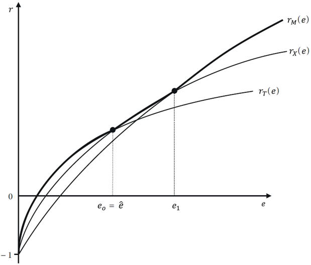
From [10] and [11] we can derive the corresponding e-r curve for commodity X. It is now convenient to plot both e-r curves for T and X together, in Figure 2.

Notice then that, in general, for each level of e, the maximum rate of profit that each sector can afford is different. If e < ê, production of sector T would be more profitable than X: The economy will specialize in the former. The opposite situation happens when e > ê. And only when e = ê, both sectors tend to co-exist. Therefore, the relevant e-r configuration is depicted by the outer envelope of the curves (thick black line).
This is enough to see the limits of the ‘light-switch’ channel. Suppose indeed that e < ê and the Central Bank decides to devalue the currency to promote sector X. Unless it exactly manages to raise e up to ê, the increased profitability of sector X will be achieved at the expense of the exclusion of sector T. The reason why this happens is the following: While both selling prices of T and X rise with the rise in e (see [5.1] and [11]), their respective costs of production do not change in the same proportion, and therefore relative costs will change. In the example of Figure 2, when e rises, X’s costs rise less than T’s, and therefore beyond the intersection of the curves, investing in X becomes more convenient than in T. So, contrary to what the “light-switch” channel asserts, devaluation will not allow, in general at least, “incorporating” new sectors in the economy (to “diversify”, so to speak, the productive structure). In other words, this policy will have both winners and losers.
Things are even more serious when there are more than two sectors, as is in Figure 3. Because in this case there will not even exist (in general) a level of e that allows the co-existence of the three sectors. Moreover, the curves may intersect more than once, as it is shown in Figure 4.

If this is the case, it may happen that both devaluation and appreciation are
able to allow, say sector X, to gain international
competitiveness. This happens when the initial level of the exchange rate
belongs to the interval
Another interesting result is the following: The idea that devaluation diversifies the productive structure means that the trade balance will be improved, the reason being that the economy will start producing (and eventually exporting) tradable commodities that were previously imported. However, the moment one realizes that a rise in e will only, if any, change the composition of the tradable sector, there is no reason that the trade balance will improve with devaluation. Suppose for instance the case in which T has a greater income elasticity than X. The rise in e shifts the productive structure towards X and exports will be less dynamic. Therefore, the trade balance will eventually deteriorate.
A final remark is worth mentioning. A basic premise for the working of both structural-change channels is that the level of r is endogenously determined by r. But consider the case in which, due to the international mobility of capital, the domestic profit rate is determined by its world-level. In this case, a currency devaluation to promote, e.g. sector X, is bound to fail. This is because the rise in e will induce an inflow of capitals that: a) either will end up appreciating the currency; or alternatively, if this inflow is sterilized by the monetary authority; b) will continue until the economy under consideration becomes the whole world supplier of X, which contradicts the assumption of a price-taking country.
4. A Price-Taker Primary Sector
Let us now consider the distributive implications when commodity T
is a primary good (“corn”), produced under “extremely favourable” conditions. The
difference with the industrial-good case is the following: Since, besides labour and
the capital goods, T is produced by a fixed factor, typically land,
if, for a given there is a positive difference between the
international price of T and its cost of production, namely
Notice then that, since the positive relationship between e and r does not longer hold (recall it was derived from [5.1]), the system gains an additional degree of freedom (there is an additional distributive variable, (, to be determined). Formally, the five-price-equation system [1]-[2]-[3]-[4]-[5.2] have the following six unknowns: E, w, r, p, pT,pNT. What this means is that, still, there remains an additional degree of freedom and, therefore, besides the inverse of money wages in foreign currency, e, another distributive variable can be determined from outside the price-system. For instance, if, due to the free mobility of capital across countries, the normal profit rate of the “small” economy under study is determined by the world level, then:
Under this closure, ( and the money prices of the tradable and non-tradable goods, and therefore, the level of the real wage, (, are endogenously determined. In this case, a rise in e decreases the real wage, but does not increase the profit rate.
Figure 5 shows the interaction among distributive variables in the presence of differential rent in sector T. Given e = ē and r = r*, the actual level of the rent can be observed in the figure, so to speak, as the difference between the maximum profit rate the sector can afford, r T (ē), and the actual profit rate, r*.

But the fact is that different closures to the one postulated by condition [12.1] can be envisaged. To name just two of the several possibilities, consider the relationship between the riskless profit rate, which we assume is equal to the interest rate set by the Central Bank and the expected rate of devaluation, as it is postulated by the interest rate parity condition.
Where ee is the expected exchange rate and e0 represents its current level. Suppose now that a rise in e introduces further volatility in agents’ perceptions about the future level of the exchange rate. In this case, it seems normal that capitalists will demand a higher profit rate to compensate for this particular kind of “risks and troubles”. We will therefore have r = r(e), with r’e > 0. Alternatively, consider next the case of given expectations regarding the future level of e. Under these conditions, a rise in e would reduce the expected rate of devaluation, and thereby, the average profit rate expected by capitalists. That is, r = r(e), with r’e < 04.
4.1. The structural change channels under differential rent
4.1.1. A shift in the composition of output
Consider first the channel that is assumed to change the composition of output in favour of sector T. The problem here is not only that, as we have seen, external demand for the tradable good has not changed, but also that devaluation cannot even persistently alter the relative profit rates in favour of sector T, since the extra-profits will be more or less quickly appropriated by land-owners under the form of differential rent.
4.1.2. The ‘light-switch’ channel
A first thing to be noticed here is that, differently from the two-industrial-goods case examined in the previous section, now it is indeed possible to develop a certain sector of the economy without in principle affecting the normal profitability of the existing ones. If, for a given e = ē, the existing sector T yields the normal profit rate, r, it is possible to determine the minimum level of e that would allow the other tradable sector (in this case, industry X) to yield this same level of the profit rate. This level, eX, is none other than the level that arises from the equalization of conditions [9.1] and [10] of the previous section:
At the level eX, both sectors would earn the same profit rate, r, and therefore could coexist (notice that, besides the normal profit rate, sector T would also earn a differential rent).
This would further seem to suggest that, for sector X to be equally profitable than sector T, devaluation of magnitude ΔeX is needed, with:
Equation [13] measures the difference between the actual level of the exchange rate and what Bresser Pereira (2008) calls the “industrial-equilibrium” exchange rate for sector X. And it seems to provide a sectorial index of competitiveness: The lower the value of ΔeX, the greater the “comparative advantages” of sector X relative to other sectors. Figure 6 shows the required rates of devaluation for two potential tradable sectors, XM and XN.

The figure shows that, to earn the profit rate
The problem for the policymaker emerges in this case when she attempts to calculate, for practical purposes, the required magnitude of devaluation for the tradable industrial sector X, since this now needs very carefully considering both the direction and magnitude of the possible interactions among distributive variables. In fact, the attentive reader may have already noticed that the magnitude of ΔeX in [13] is a function of the normal profit rate, whose behaviour, as we have seen in the previous subsection, must be ascertained case by case. Several problematic situations can be considered. For reasons of space, we will only discuss one of them.
Suppose that, besides the primary tradable sector T, there
are two industrial sectors, XM
and XN, whose respective
e - rX
curves are depicted in Figure 7. Given
the initial distributive configuration (ē,

5. A Price-Maker Tradable Sector
We now turn to consider an economy whose tradable sector determines the world price of commodity T. What this means is that commodity T’s costs of production univocally determine its price, pT6. The system of Equations [1]-[2]-[3]-[4] constitutes now the relevant conditions to determine the five unknowns: r, w, E, pNT,pT. Therefore, there is still one degree of freedom left. As in the case of production under differential rent, the profit rate is not univocally determined by e, and therefore, we can -again- consider several alternative closures, even when e is given.
5.1. A given real wage
Consider first what happens when we close the system by choosing workers’ consumption basket λ = (cT,cNT) as the numeraire:
Clearly, since the money wage is given by [3], this closure is tantamount to assuming a given real wage (. To see the effect of a rise in e, we must distinguish between two cases: The case in which the consumption basket includes both tradable and non-tradable goods (i.e. cT,cNT > 0) and the case in which workers only consume non-tradable commodities (i.e. cT = 0). In the first situation, when e rises, the whole burden of the adjustment falls on the rate of profits. In fact, if r did not fall, pT would rise, and therefore, due to [5.3], pNT would fall. But this would contradict the cost equation of the non-tradable good, because none of the terms on the right-hand side of condition [2] would have fallen.
In the case in which cT = 0, the profit rate is univocally determined by the conditions of production of good NT -conditions [2] and [5.3]-. Therefore, r does not vary with a rise in e; devaluation limits itself to raise the domestic price of commodity T due to higher costs of imported inputs. The previous effect, however, does not prevent devaluation from improving international competitiveness of sector T, since the other components of normal costs (labour and domestic capital good costs) are reduced in terms of foreign currency. The implication is that when the economy produces a tradable non-basic commodity, devaluation is fully effective in improving the competitiveness of sector T. Of course, since the economy is assumed to be a price-maker in the production of this commodity, it would not make much sense to depreciate the domestic currency to gain foreign markets. But it could be a very effective policy to close a competitiveness gap of a particular sector that is initially excluded from international trade. We will come back to the limits to this policy below (see section 5.4).
5.2. A given profit rate
Alternatively, one could fix the profit rate from outside the system. Formally, we must replace condition [5.3] by the following condition:
Where
5.3. Distributive conflict among open economies
The case of a given profit rate is a useful starting point to examine a final possible closure of the system, in which the profit rate and the real wage are both given. Of course, this kind of closure would be unconceivable within a closed economy, and therefore, it forces us to consider distributive interactions between the domestic economy and the rest of the world.
To formalize this interaction, we must eliminate condition [3] and introduce an equation that endogenously determines the nominal wage to satisfy a certain real wage target, ϖ. This can be done by re-expressing condition [9.1] as:
Therefore, the price system is composed of Equations [1]-[2]-[4]-[9.2]-[5.4]. Suppose now that there is a rise in e. For an initially given nominal wage, domestic prices will rise to preserve the level of the normal profit rate. However, since this will decrease the real wage, nominal wages must rise to restore the target level of (. Therefore, if there is full wage resistance, devaluation fails to alter income distribution and simply modifies the nominal scale of the system.
More interesting is to consider the effect of an exogenous rise of one of the domestic distributive variables, either r or (. In this case, the fact that the other distributive variable is given means that the whole burden of the adjustment falls on foreign income distribution. If, due to the free mobility of capital across countries, the domestic and international profit rates tend to coincide, one should expect a fall in the foreign real wage, (*, which is materialized through an improvement of the terms of trade faced by the domestic economy. In fact, when for instance, ( goes up, domestic prices must also rise. Otherwise, the domestic profit rate would fall. And for a given nominal exchange rate, prices in foreign currency will also increase. In other words, the country “exports inflation”, which erodes the purchasing power of foreign workers.
This interaction can be described by means of Figure 8. The left-hand side of the figure shows the standard negative relationship between the real wage, which for simplicity is entirely expressed in terms of commodity T, and the profit rate. The rise in ω acts as a technical improvement that allows increasing the domestic real wage without decreasing domestic profitability. This is shown by a shift to the right of the (-r curve. Symmetrically, on the right-hand side of the figure, we show a movement along the ω-ω* curve, which is the expression of the distributive conflict between domestic and foreign workers8. This outcome resembles the interaction between the so-called “imperialist” and “dependent” countries that has been carefully studied by some Latin American structuralist scholars (see, for instance, Braun, 1973).

5.4. Structural change in a price-maker economy
Consider an initial situation in which the supply price of commodity T in foreign currency is greater than its internationally given price. In other words, the following condition holds:
Under these circumstances, the domestic economy could use devaluation policy to revert the sign of the inequality and, therefore, become the new price-maker of commodity T. Appealing and simply as this policy seems to be, it faces several limitations. First, unless workers do not consume commodity T, devaluation will increase the price of the wage basket, and therefore, the possibility of strong wage resistance cannot be excluded a priori. Second, and perhaps more importantly, with this policy the economy in questions would have gained market share only at the expense of foreign competitors, since there is no reason to expect nothing but a minor increase in global demand for T. In other words, it is most likely that through devaluation, the domestic economy would have exported unemployment. Considering that most countries have exchange rate policy as one of their policy options, one should expect that competitors devalue their own currencies as well, thereby starting a currency war that ends up in a zero-sum game.
6. Concluding Remarks
Along this article we have examined the interaction among distributive variables under three different productive structures: Price-taking economies that produce tradable industrial goods, price-taking countries that produce a primary good under differential rent and, finally, price-making countries. It may be useful now to summarize the main results of the article.
In the first place, we have shown that none of the mechanisms that are argued to induce structural change through a rise in the real exchange rate is sufficiently general. First, when the economy is price-taker in the production of industrial goods, diversification of the productive structure will not generally be possible, the usual case being that the competitiveness of one tradable sector is gained at the expense of the other tradable sectors of the economy. Neither will it be generally possible to use devaluation to shift the composition of output in favour of the tradable sectors, since the arguments adduced for that conclusion usually assume some kind of Say’s Law. Second, when the economy produces a primary good under conditions of differential rent, diversification will be possible, but this requires a careful consideration of the interaction among distributive variables, not only the direction of this interaction, but also its magnitude. Finally, while from a theoretical point of view, devaluation may succeed in making an economy a price-maker of a particular sector, trading partners will most likely react through competitive devaluations which may end up in a zero-sum game.
In the second place, we have also shown the different effects of devaluation on income distribution. Within a price-taking country that produces industrial goods, devaluation will generally raise the general profit rate and reduce the real wage. This is not generally true, neither when the economy produces primary goods under conditions of differential rent, nor when is a price-maker of the tradable good. In economies producing primary goods, it could well happen that devaluation increases the magnitude of the rent at the expense of both the real wage and the average profit rate. Moreover, one could even think of situations in which the whole burden of the adjustment falls on the profit rate; although this does not seem to be very likely the moment the free mobility of capital across countries is duly considered. What the consideration of a price-making economy adds to the previous case is the possibility that the economy exports inflation to its trading partners, at least within some ranges, by raising either the domestic real wage or the profit rate.
Taken together, these two main results of the paper, namely: 1) the absence of general connections between devaluation and structural change, and 2) the richness of the possible interactions among distributive variables, strongly suggest that the outcomes of devaluation, both in terms of its effects on the productive structure and on income distribution, should be very carefully considered before this policy is recommended to induce structural change.

